| Term / Concept | Definition / Explanation |
|---|---|
| Normal Distribution | A continuous probability distribution shaped like a smooth, symmetric bell curve. Fully described by two parameters: mean (μ) and standard deviation (σ). Many naturally occurring measurements approximate this distribution. |
| Role of μ and σ | • μ determines the centre of the distribution. • σ controls the spread: larger σ means a wider, flatter curve; smaller σ means a narrower, steeper curve. |
| Empirical Rule (68–95–99.7) | Approximately: • 68% of values lie within μ ± σ • 95% lie within μ ± 2σ • 99.7% lie within μ ± 3σ |
| Normal Probability Calculations | Probabilities of the form P(X < a), P(a < X < b), P(X > b) are found using technology. Students do not use standardisation to z; calculators handle all computations directly. |
| Inverse Normal | Used to find the value x such that a given proportion of the data lies below x. Calculator inputs typically require: area (probability), mean μ and standard deviation σ. No z-score transformations are required in the SL course. |
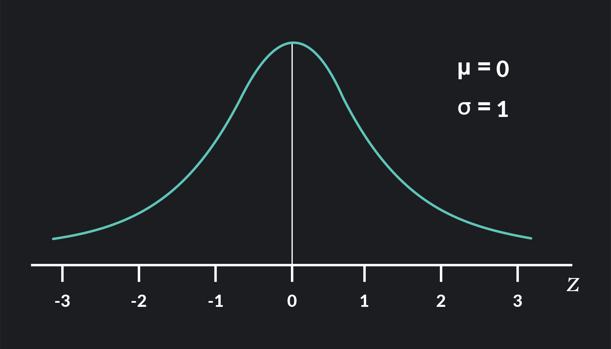
1. The Normal Distribution and Curve
The normal distribution is a continuous probability distribution with a characteristic
bell-shaped curve. A normal random variable X is written as X ~ N(μ, σ), where:
- μ = mean (centre of the distribution)
- σ = standard deviation (measure of spread)
- The curve is perfectly symmetric about x = μ.
- The highest point (peak) of the curve occurs at x = μ.
- Total area under the curve = 1 (represents probability 1).
Unlike discrete distributions (such as binomial), the normal distribution is
continuous. Probability is represented by area under the curve, not by bars.
For a single exact value P(X = a) = 0; we always consider intervals such as P(a < X < b).
Many real-life measurements are approximately normal:
- Human heights and masses within a population
- IQ scores and some psychological test scores
- Measurement errors in experiments
- Natural variation in manufacturing processes
Recognising when the normal model is reasonable allows us to make powerful probability-based predictions.
2. Key Properties & the 68–95–99.7 Rule
Important qualitative properties:
- Shape is bell-shaped and symmetric about μ.
- As x moves far from μ, the curve approaches (but never touches) the x-axis.
- Mean, median and mode are all equal to μ.
For many normal distributions, the following empirical rule holds:
- Approximately 68% of data lies between μ ± σ.
- Approximately 95% lies between μ ± 2σ.
- Approximately 99.7% lies between μ ± 3σ.
These percentages provide a quick way to judge whether a value is “typical” or “unusual”.
Values beyond μ ± 2σ are uncommon; beyond μ ± 3σ are very rare in a normal distribution.
When a question asks whether a data value is “unusual” or “consistent with the model”,
compare it to μ ± 2σ or μ ± 3σ and comment using the 68–95–99.7 rule.
A brief sentence such as “this lies more than 2σ from the mean, so it is unlikely” often earns reasoning marks.
3. Diagrammatic Representation
In exam diagrams:
- Draw a smooth bell-shaped curve over the x-axis.
- Mark the mean μ on the horizontal axis at the centre.
- Optionally mark μ − σ, μ + σ, μ − 2σ, μ + 2σ to show the spread.
- Shade the region corresponding to the probability being asked, e.g. x > a or a < x < b.
Even when the question uses technology, a quick sketch with a shaded region helps you
understand what the GDC output represents and can reveal obvious mistakes (like probabilities > 1 or negative).
4. Normal Probability Calculations (Using Technology)
To work with a normal variable X:
- Define the variable clearly:
“Let X be the height (in cm) of students in a school, X ~ N(170, 8).” - Sketch a quick normal curve marking μ and shading the relevant region.
- Use GDC normal distribution functions to find the area (probability).
Common probability types:
- P(X < a) → lower tail
- P(X > a) = 1 − P(X < a) → upper tail
- P(a < X < b) = P(X < b) − P(X < a)
Example 1 – Tail probability
Suppose X ~ N(100, 15). Find P(X > 130).
- Sketch: mean at 100, shade the right tail beyond 130.
- Use your calculator’s normal CDF function with mean = 100, sd = 15, lower = 130, upper = a large number (e.g. 109).
- Result is a small probability showing such a high value is rare.
- For P(X < a), use lower = −109, upper = a.
- For P(X > a), use lower = a, upper = 109.
- For P(a < X < b), use lower = a, upper = b.
- Always double-check that your shaded sketch matches the bounds you entered.
Clearly state whether the area you enter is left tail or right tail.
If the question gives a right-tail probability (P(X > x) = p), convert to a left-tail area first: P(X < x) = 1 − p.
5. Inverse Normal Calculations
Inverse normal problems ask for a value of X corresponding to a given area (probability).
The mean μ and standard deviation σ are given, and we find x such that:
P(X < x) = p or P(X > x) = p or P(a < X < b) = p.
You do not need to transform to the standardised variable z in IB exams;
use the inverse normal function on your GDC directly with μ and σ.
Example 2 – Percentile
Test scores are normally distributed with mean 60 and standard deviation 8.
Find the score that marks the top 10% of students.
- We want the 90th percentile, since 10% are above and 90% are below.
- So find x such that P(X < x) = 0.90.
- Use inverse normal with area = 0.90, mean = 60, sd = 8 → x ≈ 70.2
- Interpretation: students scoring about 70 or above are in the top 10%.
The normal distribution is a model, not reality. Important questions:
- When is it reasonable to assume data are normal, and who decides?
- What happens if we apply the normal model where it does not hold (e.g. income distributions)?
- How do choices about which data to include or exclude influence the “fit” to a normal curve?
Misuse of the normal model can lead to misleading or dangerous conclusions, especially in medicine and social policy.
📌 Practice Questions — Normal Distribution
Multiple Choice Questions
MCQ 1. A random variable X follows a normal distribution with mean μ and standard deviation σ.
Which statement is always true?
A. P(X = μ) > 0
B. The total area under the curve equals μ
C. The distribution is symmetric about x = μ
D. Exactly 95% of values lie between μ ± σ
Answer & Explanation
Correct answer: C
A normal distribution is perfectly symmetric about its mean μ, meaning values equally far above and below μ
have equal probability.
For continuous distributions, P(X = μ) = 0, not greater than 0.
The total area under the curve equals 1, not μ.
The 95% rule applies to μ ± 2σ, not μ ± σ.
MCQ 2. Heights of students are normally distributed with mean 170 cm and standard deviation 6 cm.
Approximately what percentage of students have heights between 164 cm and 176 cm?
A. 34%
B. 68%
C. 95%
D. 99.7%
Answer & Explanation
Correct answer: B
The interval 164 to 176 corresponds to μ ± σ (170 ± 6).
By the 68–95–99.7 empirical rule, approximately 68% of values lie within one standard deviation of the mean.
MCQ 3. For a continuous random variable X, which statement is correct?
A. P(X = a) can be calculated using the pdf
B. Probabilities are represented by areas under the curve
C. The probability distribution is shown using bars
D. Individual outcomes have non-zero probability
Answer & Explanation
Correct answer: B
For continuous random variables, probabilities are represented by areas under the probability density curve.
The probability of any single exact value is zero, and bar charts are used only for discrete variables.
Medium-Length Questions
Question 1.
The reaction time (in seconds) of a group of drivers is normally distributed with mean 0.8 and standard deviation 0.1.
(a) Find the probability that a randomly selected driver has a reaction time greater than 0.95 seconds.
(b) Explain, using the context, whether a reaction time of 1.05 seconds would be considered unusual.
Answer & Explanation
(a)
Let X be the reaction time.
X ~ N(0.8, 0.1).
We calculate P(X > 0.95).
Using technology, this corresponds to the upper tail beyond 0.95.
Since 0.95 is 1.5 standard deviations above the mean, the probability is relatively small.
(b)
A reaction time of 1.05 seconds lies 2.5 standard deviations above the mean:
(1.05 − 0.8) ÷ 0.1 = 2.5
Values more than 2σ from the mean are uncommon, and those beyond 3σ are very rare.
Therefore, 1.05 seconds would be considered unusual but not impossible under the normal model.
Question 2.
Exam scores are normally distributed with mean 60 and standard deviation 8.
(a) Find the score that separates the lowest 20% of students from the rest.
(b) Interpret your answer clearly in context.
Answer & Explanation
(a)
We want the 20th percentile, so we find x such that P(X < x) = 0.20.
Using inverse normal with mean 60 and standard deviation 8 gives:
x ≈ 53.3
(b)
This means that approximately 20% of students score below 53.3, while the remaining 80% score above this value.
The score 53.3 therefore represents a lower-performance threshold in the distribution.