AHL 2.8 — TRANSFORMATIONS OF GRAPHS

📌 Understanding Transformations

• The base function y = f(x) represents the original untransformed graph, which acts as the reference shape before any movement, stretching, shrinking, or reflection is applied to it.
• A transformation is a mathematical operation that moves or reshapes a graph while preserving its fundamental structure, such as translations, reflections, and stretches.
• The coordinate axes remain fixed and invariant during transformations, meaning all movements are measured relative to these stationary reference lines.
• Translations are often written using vector notation (a, b), where a controls horizontal motion and b controls vertical motion of the entire graph.

📌 Translations — Shifting Graphs

• The transformation y = f(x) + b moves every point on the graph vertically by b units, upward if b is positive and downward if b is negative.
• Example: y = x² + 4 moves the parabola four units upward without altering its width or orientation.
• The transformation y = f(x − a) moves the graph horizontally, shifting it right by a units if a is positive and left by a units if a is negative.
• Example: y = √(x − 2) shifts the square-root graph two units to the right.
• The combined transformation y = f(x − a) + b applies both shifts using the translation vector (a, b).
• Example: y = (x − 3)² − 2 shifts the parabola three units right and two units downward.

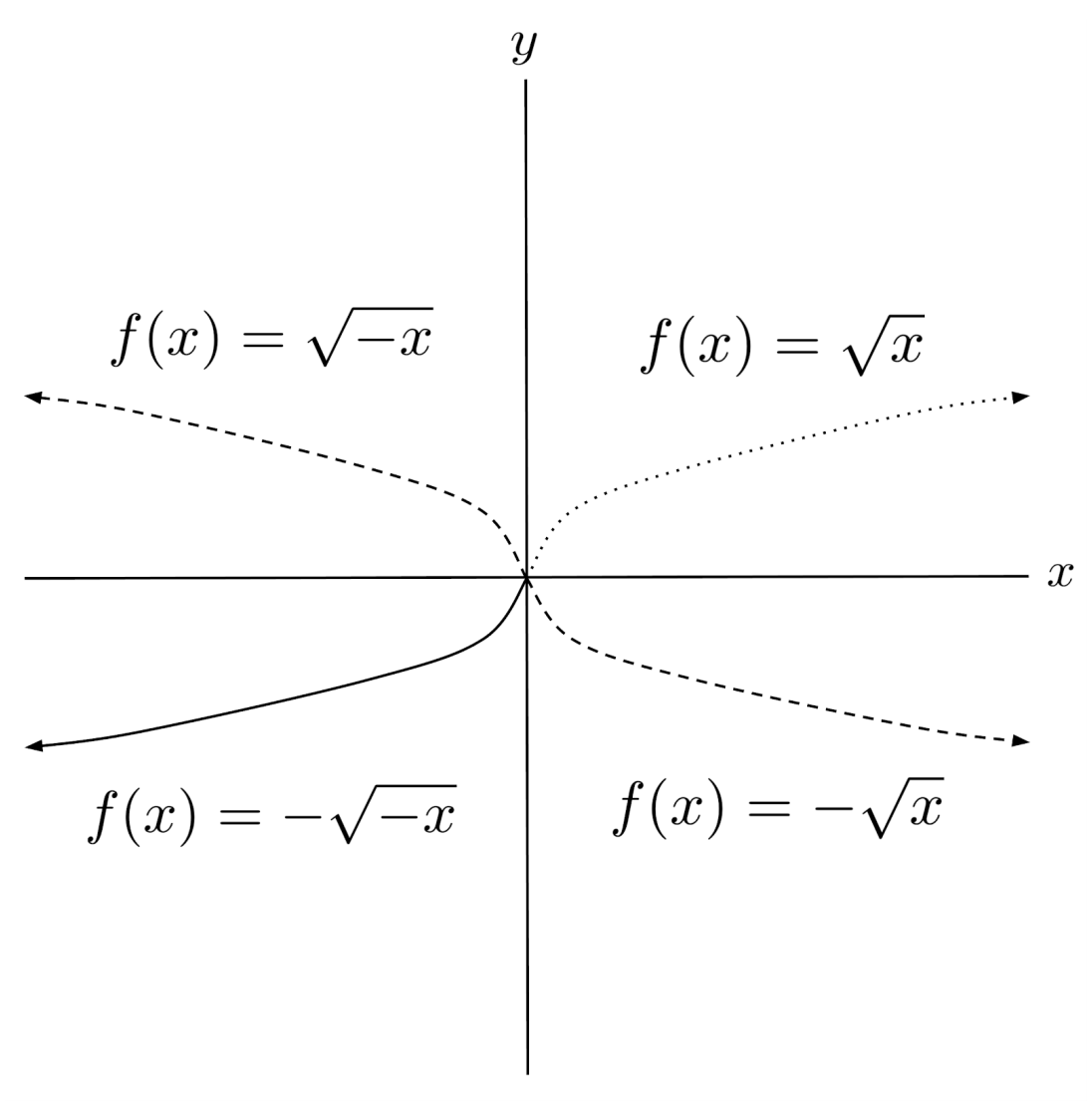
📌 Reflections — Flipping Graphs

• The graph y = −f(x) reflects the original curve across the x-axis, reversing all vertical values while preserving horizontal positions.
• Example: y = x² becomes y = −x², changing an upward-opening parabola into a downward-opening one.
• The transformation y = f(−x) reflects the graph across the y-axis, producing a horizontal mirror image of the original curve.
• Example: y = eˣ becomes y = e⁻ˣ, reversing its growth direction while maintaining exponential behavior.

reflections-of-functions-1.png

📌 Stretches — Scaling Graphs

• Vertical stretches are written as y = p·f(x), multiplying all y-values by p, which changes amplitude or vertical height without altering the x-structure.
• Example: y = 2 sin x doubles the wave’s amplitude while keeping the same period.
• Horizontal stretches take the form y = f(qx), compressing the graph horizontally when q > 1 and stretching it when 0 < q < 1.
• Example: y = sin(2x) halves the original period of the sine curve.

Compression-and-Stretching-1.webp

📌 Composite Transformations — Multiple Changes

• Composite transformations involve applying more than one transformation sequentially, producing graphs that combine stretching, reflection, and translation together.
• The order of transformations is critical: horizontal changes inside f( ) must always be applied before vertical transformations outside f( ).
• Example: y = x² → y = 3x² applies a vertical stretch of factor 3 → y = 3x² + 2 shifts the graph upward two units.
• Example: y = sin x → y = 4 sin(2x) doubles frequency and quadruples amplitude.

📌 Common Misconceptions

• Horizontal transformations behave opposite to intuition, meaning y = f(x − 2) shifts right rather than left.
• Vertical transformations behave intuitively, meaning y = f(x) + 3 always shifts upward by three units.
• Altering the order of composite transformations can completely change the final position and shape of the graph.

🔢 GDC & Technology Integration

• Use your GDC to compute compositions directly by defining f(x) and g(x), then evaluating f(g(x)).
• When finding inverses, use the GDC to verify correctness by checking that (f ∘ f⁻¹)(x) = x numerically.
• For quadratic inverses with restrictions, graph both f and f⁻¹ to visually confirm mirror symmetry across y = x.
• Always record the algebraic working — calculator output alone is not awarded full method marks.

🌍 Real-World Connection

Composite functions appear in pricing chains (cost → tax → discount),
unit conversion pipelines, and physics (displacement → velocity → acceleration).
Each stage depends strictly on the previous output.

📝 Paper Strategy

• Always write compositions in the correct inside → outside order: f(g(x)), never f(x)g(x).
• When finding inverses, you must explicitly show the swap of x and y before solving.
• If the function is not one-to-one, you must state the domain restriction clearly or you lose accuracy marks.
• Final answers must be labelled properly as f⁻¹(x), not just “y = …”.

📝 Paper Strategy

• Always state the restricted domain with your inverse.
• Verify inverses using (f ∘ f⁻¹)(x).
• Never assume composition order can be swapped.
• Method marks come from clean algebra — not calculator output.

SL 2.5: MODELLING WITH FUNCTIONS

In this topic we learn how different function families can be used to describe real situations, how each parameter changes
the graph’s shape, and how we can interpret solutions in context rather than treating them as abstract algebraic answers.

📌 Linear models — f(x) = mx + c

Meaning of parameters

• The parameter m represents the constant rate of change, showing how much the output increases or decreases
  whenever the input rises by exactly one unit, which is why it is often described as the slope.
• The parameter c gives the function value when x = 0, meaning it represents the starting
  amount or fixed fee in many word problems, and it always appears as the y-intercept on the graph.

Graph behaviour

• Linear graphs are always straight lines because the change in y for each equal change in x is constant, so there is no
  curvature and the gradient is the same everywhere along the line.
• A positive value of m produces an increasing line that slopes upwards from left to right, whereas a negative value of m
  produces a decreasing line, sloping downwards as x increases across the horizontal axis.

Worked example – taxi fare

A taxi charges according to the model F(x) = 60 + 15x, where F is the fare in rupees and x is the distance
travelled in kilometres. The term 60 represents a fixed base charge, while 15 is the cost per kilometre added on top.

Suppose the total fare is ₹180. To find the distance travelled, we solve the equation
60 + 15x = 180. Subtracting 60 from both sides gives 15x = 120, and dividing by 15 gives
x = 8. Therefore, the passenger travelled 8 km according to this linear pricing model.

📌 Quadratic models — f(x) = ax² + bx + c

Meaning of parameters

• The coefficient a controls whether the parabola opens upwards or downwards and how “narrow” it is; large
  values of |a| make the curve steeper and more compressed, while small values make it flatter and more spread out.
• The coefficient b influences the horizontal location of the vertex, because the x-coordinate of the
  turning point is always x = −b ÷ (2a), so changing b shifts the vertex left or right along the axis.
• The constant term c gives the y-intercept of the graph, meaning it tells us the value of the function
  when x is zero and often represents an initial height, starting cost, or baseline quantity in applications.

Graph behaviour and vertex

• If a > 0 the parabola opens upwards and the vertex represents a minimum value, which is frequently
  interpreted as a lowest cost, minimum height, or smallest possible value that the model can attain.
• If a < 0 the parabola opens downwards and the vertex becomes a maximum value, which is essential in
  contexts such as maximum profit, maximum height of a projectile, or maximum area enclosed by a fence.

Worked example – f(x) = x² − 6x + 5

We can factor the quadratic expression x² − 6x + 5 as (x − 1)(x − 5), which immediately
reveals that the function has zeros at x = 1 and x = 5, giving the x-intercepts of the
graph where the output value becomes zero.

To find the vertex, we compute x_v = −b ÷ (2a) = −(−6) ÷ (2 × 1) = 6 ÷ 2 = 3. Substituting this
into the function gives f(3) = 3² − 6·3 + 5 = 9 − 18 + 5 = −4, so the parabola has a minimum point at
(3, −4).

Therefore the graph is a U-shaped curve opening upwards, crossing the x-axis at 1 and 5, with its lowest point at x = 3,
where the function value equals −4, which is useful when describing minimum distance or minimum cost.

📌 Exponential models — f(x) = k aˣ + c or f(x) = k eʳˣ + c

Meaning of parameters

• The constant k sets the initial scale of the model, since the value at x = 0 is always f(0) = k + c,
  meaning it often corresponds to the starting population, initial amount of substance, or initial balance in a financial account.
• The base a or exponential rate r determines how quickly the quantity grows or decays; values
  with a > 1 or r > 0 represent growth, whereas 0 < a < 1 or
  r < 0 correspond to exponential decay.
• The constant c represents a horizontal asymptote, meaning it gives the long-term baseline value that the
  model approaches but rarely reaches, such as background temperature or minimum population level.

Worked example – continuous growth

Consider the population model P(t) = 100 e^0.03t, where t is measured in years. The value 100 is the
starting population, while the exponent 0.03 represents a continuous annual growth rate of three percent.

To find the population after ten years we calculate P(10) = 100 e^0.30. Evaluating the exponential
gives approximately e^0.30 ≈ 1.3499, so the population is about 135 individuals,
meaning the size has increased by roughly thirty-five percent over the ten-year period.

📌 Direct and inverse variation — f(x) = a xⁿ and f(x) = a ÷ xⁿ

Interpretation

• In direct variation, the output is proportional to a power of the input, so multiplying the input by a
  constant factor multiplies the output by a predictable power of that factor, which explains scaling behaviour in physics
  and geometry.
• In inverse variation, the output decreases when the input increases because the quantity is divided by a
  power of x, and the graph normally has a vertical asymptote at x = 0, showing that certain values of x are not allowed.

Worked example – pressure and volume

Suppose gas pressure P is inversely proportional to volume V according to P = k ÷ V. If the pressure is 2 units
when the volume is 3 litres, then k = 2 × 3 = 6. For a volume of 5 litres, the pressure becomes
P = 6 ÷ 5 = 1.2, illustrating how increasing volume reduces pressure.

📌 Cubic models — f(x) = a x³ + b x² + c x + d

Behaviour of cubic graphs

• Cubic functions often produce S-shaped curves with one point of inflection and up to two turning points, allowing them to
  model situations where a quantity initially increases, then decreases, and finally increases again.
• The sign of a determines the end behaviour; if a > 0 the graph falls to the left and rises to the
  right, while if a < 0 it rises to the left and falls to the right as x becomes very large in magnitude.

Worked example – f(x) = x³ − 6x² + 11x − 6

Trying simple integer values, we find f(1) = 0, so (x − 1) is a factor. Dividing gives
f(x) = (x − 1)(x² − 5x + 6), and factorising the quadratic yields
f(x) = (x − 1)(x − 2)(x − 3), so the cubic has real roots at 1, 2 and 3.

Differentiating gives f′(x) = 3x² − 12x + 11. Solving f′(x) = 0 produces turning points near x ≈ 1.42 and
x ≈ 2.58, indicating where the graph switches between increasing and decreasing, which is important when analysing maximum
or minimum output levels.

📌 Sinusoidal models — f(x) = a·sin(bx) + d or a·cos(bx) + d

Meaning of parameters

• The amplitude a is the distance from the midline to a peak or trough and represents the maximum deviation
  from the average level, such as the greatest change from mean temperature in a daily or seasonal cycle.
• The coefficient b controls the period, since period = 2π ÷ b (or 360° ÷ b in degrees), meaning larger
  values of b cause the wave to repeat more frequently over the same horizontal distance.
• The constant d shifts the entire graph vertically and marks the midline; it represents the average value
  around which the oscillations occur, such as mean temperature, average daylight length, or constant voltage level.

Worked example – temperature model

Consider T(t) = 10 sin((π/6)t) + 20, where t is time in hours. The amplitude 10 means temperatures oscillate
10 degrees above and below the mean, and the vertical shift 20 indicates an average temperature of 20°C.

The period is 2π ÷ (π/6) = 12 hours, so the full warm-cool cycle repeats every twelve hours. The maximum
occurs when the sine term equals 1, which happens when (π/6)t = π/2, giving t = 3 hours, so the maximum temperature is
30°C at t = 3.

📌 Key features of graphs — systematic approach

1. Intercepts: Substitute x=0 (for y-intercept) and y=0 (for x-intercepts).
2. Symmetry: Test if f(−x) = f(x) or f(−x) = −f(x).
3. Vertex: For y = ax² + bx + c, vertex = (−b ÷ 2a, f(−b ÷ 2a)).
4. Extrema: Local maximum/minimum identified via vertex (quadratic) or using graphing technology (for non-quadratic).
5. Asymptotes: Check denominator = 0 (vertical), and limits as x → ±∞ (horizontal/oblique).
6. End behaviour: Examine leading term of f(x) for general trend as x → ±∞.

📌 Finding intersection points

• Analytically: Solve f(x) = g(x) → gives x-coordinate(s) of intersection; substitute back to find y.
• Using technology: Use “intersect” or “solve” functions on GDC to find intersection coordinates quickly.
• Interpreting intersections:
  • In economics: market equilibrium → demand = supply.
  • In physics: time when two objects are at same position.
  • In geography: intersection of contour curves represents equal elevation points.

📌 Purpose: Learn what a graph shows, how to sketch a function from algebraic info or a screen, what features to label, and how to use technology to graph functions and their sums/differences. Emphasis on clarity: every sketch must label axes and key features and justify choices.

📌 Sketching principles — what to include and why

• Label both axes and include scale marks where relevant.
• Always mark and label: intercepts, turning points (approximate coordinates), vertical & horizontal asymptotes (equations), and any discontinuities (open/solid circles).
• State whether the sketch is exact or approximate (sketch). If transferring from screen to paper, note the scale you used.

• Use arrows on ends to indicate end behaviour when graph continues beyond drawn region (e.g., y → ∞ as x → ∞).

📌 Creating a sketch from algebraic or contextual information

1. Identify domain/range & continuity: look for roots, denominators, square roots, logs and their restrictions.
2. Find intercepts: set x = 0 for y-intercept, solve f(x) = 0 for x-intercepts (approximate if needed).
3. Find turning points (if easy): for simple polynomials use calculus (f′(x)=0) or symmetry for quadratics. For SL, approximate coordinates are sufficient if labelled.
4. Locate asymptotes: vertical where denominator 0 (and limit → ±∞), horizontal/oblique from end behaviour (limits as x → ±∞).
5. Combine the info into shape: sketch curve, label features and indicate approximate coordinates or equations (e.g., x = 2, y = −1).

📌 Examples & real situations

📌 Sketching sums & differences — practical method

• Use table-of-values for f and g at same x-values, compute f ± g pointwise, then plot or use GDC to plot f+g directly.
• When sketching by hand, choose 6–8 representative x-values (including turning points and intercepts) and connect smoothly.
• Label points used (e.g., x = 0, ±1, turning points) so examiner sees your method.

📌 Practice questions (sketch & interpret)

1. Sketch: y = x² − 4x + 3. Show vertex, intercepts and axis of symmetry. State domain & range.
2. Sketch & transfer: Plot f(x) = tan x in region x ∈ (−π/2, π/2). Label asymptotes and key points; transfer the central branch to paper using table-of-values.
3. Sums: Given f(x) = e^−x and g(x) = 0.5, sketch f and g and then sketch f + g. Explain how addition changes end behaviour.
4. Context: A city’s traffic flow vs time is modelled as a periodic curve plus a linear trend. Sketch a plausible shape and explain turning points in context.

📌 Quick sketch checklist

• Axes labelled, scale marked, and units (if any) shown.
• Intercepts and approximate coordinates of turning points labelled.
• Asymptotes drawn with equations (dashed lines) and discontinuities shown as open circles.
• State whether sketch is exact or approximate; include 2–4 reference points used to draw the curve.