Author: Admin

  • SL 4.3 – Measures of Central Tendency and Dispersion

    This topic covers numerical summaries of data, including measures of central tendency, dispersion,
    and the effects of changing data values. These tools help us understand distribution shapes, compare
    two datasets, and evaluate the reliability of conclusions drawn from sample data.

    1. Measures of Central Tendency

    Mean

    The mean is calculated by summing all values and dividing by the number of items. It is highly
    sensitive to extreme values, meaning it works best for fairly symmetrical distributions.

    Median

    The median represents the middle value of a sorted dataset. Since it is unaffected by outliers or
    large extreme values, it is an appropriate measure for skewed distributions.

    Mode

    The most frequent value in the data. Especially useful for categorical or discrete data.

    🌍 Real-World Example:
    Income data is typically summarised using the median, not the mean,
    because a few very high earners can distort the average.

    Estimation of Mean from Grouped Data

    For grouped data, mid-interval values are used as representatives. Multiply each midpoint by its
    frequency, sum these products, and divide by the total frequency to estimate the mean.
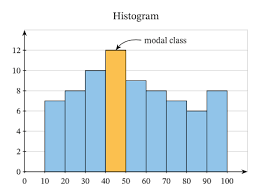
    2. Modal Class

    For grouped data with equal intervals, the modal class is the class with the highest frequency.
    This is useful when exact data values are not available.

    444 × 339

    3. Measures of Dispersion

    Interquartile Range (IQR)

    The IQR measures the spread of the middle 50% of the data. It is resistant to outliers and gives a
    clearer picture of the central distribution’s variability.

    Variance and Standard Deviation

    Variance measures the average squared deviation from the mean. The standard deviation, its square root,
    measures the typical distance from the mean and is widely used for statistical comparison.

    🌍 Real-World Example:
    In sports analytics, standard deviation measures consistency.
    An athlete with a low SD performs reliably across games.

    4. Effect of Constant Changes

    • Adding a constant to all data values shifts the mean by that constant but does not change the standard deviation.

    • Multiplying all values by a constant multiplies both the mean and the standard deviation by that constant.

    🧠 Examiner Tip:
    Students often forget that adding or subtracting a constant does not change the
    spread of data. Only multiplication affects spread.

    5. Quartiles of Discrete Data

    Quartiles divide data into four equal parts. Different calculators may use different algorithms, so results
    may differ slightly between hand calculation and GDC output.

    🟢 GDC Tip:
    When using a calculator to compute quartiles or standard deviation, always write
    “Using GDC” in your work to show that you are aware of algorithmic differences.

    🔍 TOK Perspective:
    Why do multiple formulas for variance exist? Does this imply that mathematical truth can have
    multiple valid representations?

    📊 IA Suggestion:
    Investigate whether different sports, cities, or environmental datasets show greater variability.
    Justify your choice of mean, median, IQR, and SD in your analysis.

    ❤️ CAS Connection:
    Collect real data during a community activity (fitness, volunteering outputs, environmental waste)
    and analyse its central tendency and spread as part of CAS reflections.

  • SL 4.2 — Presentation of Data and Distribution Diagrams

    This topic focuses on how to organise and display data so that patterns,
    clusters and outliers can be seen clearly. You should understand how to construct and interpret
    frequency tables, histograms, cumulative frequency graphs and box-and-whisker diagrams.

    Frequency distributions (tables)

    Discrete and continuous data

    For discrete data (for example, number of goals, number of siblings), each distinct value can be
    listed along with its frequency.
    For continuous data (for example, height, reaction time), individual values are grouped into
    class intervals, such as 150 ≤ height < 160.

    Class intervals and frequency

    A frequency distribution table shows:

    • each value or class interval, and
    • the corresponding number of observations (frequency).

    In IB exams, class intervals are usually given as inequalities without gaps,
    ensuring that every data value belongs to exactly one class.

    🌍 Real-world connection

    Frequency tables are used in sciences (for recording repeated measurements),
    economics (income brackets), and social sciences
    (age groups, survey responses). They are often the first step before creating
    histograms or box plots.

    Histograms

    Basic idea

    A histogram is a diagram used mainly for continuous data.
    Along the horizontal axis we show the class intervals; along the vertical axis we show the
    frequency. Each class interval is represented by a bar whose height equals its frequency.
    In this course you only need frequency histograms with equal class widths
    (frequency density histograms are not required).

    Reading a histogram

    • The shape shows whether the distribution is symmetric, skewed, unimodal or bimodal.
    • The highest bars indicate where data values are most common.
    • Very low or isolated bars may indicate outliers or rare events.

    🌍 Real-world connection

    Histograms are widely used to check whether data may be approximately
    normally distributed, for example when analysing test scores,
    measurement errors in physics experiments, or daily returns in finance.

    Cumulative frequency and cumulative frequency graphs

    Cumulative frequency

    The cumulative frequency for a class is the total number of data values
    up to and including that class. It shows how many observations lie below a given boundary.

    To construct a cumulative frequency table, add frequencies progressively down the table.
    For grouped data, use the upper class boundary of each class.

    Cumulative frequency graph

    A cumulative frequency graph plots cumulative frequency (vertical) against the upper class boundary (horizontal).
    You then join the points with a smooth curve or straight line segments.

    From the graph you can estimate:

    • Median: point where cumulative frequency is half of the total.
    • Lower quartile (Q1): cumulative frequency at 25% of total.
    • Upper quartile (Q3): cumulative frequency at 75% of total.
    • Percentiles: e.g. the 90th percentile where 90% of data lie below.
    • Range and interquartile range (IQR): read approximate minimum, maximum, Q1, Q3 from the graph.

    📊 IA spotlight

    Cumulative frequency graphs are excellent for comparing two groups, such as
    reaction times of different age ranges or test scores of two different classes.
    You can use medians and quartiles from ogives to comment on central tendency and
    spread in your Internal Assessment.

    Box-and-whisker diagrams

    Constructing a box plot

    A box-and-whisker diagram (box plot) summarises a distribution using
    five key values:

    • Minimum value (or lower end, excluding outliers),
    • Lower quartile Q1,
    • Median,
    • Upper quartile Q3,
    • Maximum value (or upper end, excluding outliers).

    The box spans from Q1 to Q3 and contains the middle 50% of data.
    The whiskers extend to the minimum and maximum non-outlier values.
    Any outliers (more than 1.5×IQR from the nearest quartile) are shown with a cross.

    Comparing distributions with box plots

    Box plots are particularly useful for comparing two or more data sets.
    When comparing, comment on:

    • Median: which group tends to have higher or lower values?
    • IQR: which group has more variation in the middle 50% of data?
    • Range: how wide is the entire spread?
    • Symmetry: is the median centred in the box (approximately symmetric) or closer to one side (skewed)?
    • Outliers: are there any extreme values that may affect interpretation?

    🔍 TOK perspective

    Box plots compress large data sets into just a few numbers.
    This makes patterns easier to see, but also hides detail.
    To what extent does summarising data improve understanding, and to what extent might it
    oversimplify reality?

    Indications of normality

    A roughly symmetric box plot, where the median is near the centre of the box and the whiskers are of
    similar length, suggests that the data may follow a distribution close to normal.
    Strong skewness or several outliers indicate that the data are unlikely to be normally distributed.

    🌍 Connection to other subjects

    In science, histograms and box plots summarise laboratory measurements;
    in geography, they model rainfall or population data;
    in business and economics, they are used to present income distributions,
    sales figures and risk.

    🧠 Examiner tip

    • Always label axes clearly and show class boundaries for histograms and cumulative frequency graphs.
    • When comparing box plots, refer specifically to median, IQR, range and any outliers instead of vague phrases like “more spread out”.
    • Check that your frequencies add up to the total number of data values.

    📱 GDC use

    • Use the statistics menu of your GDC to generate histograms, cumulative frequency graphs and box-and-whisker plots quickly.
    • Let the GDC compute quartiles, median and IQR, then sketch neat graphs by hand in exams if technology is not allowed.
  • SL 4.1 — Introduction to Statistical Concepts and Sampling

    Key Statistical Concepts

    This topic introduces the foundational language and ideas used in statistics. Students must understand the
    difference between populations and samples, types of data, and potential sources of bias when interpreting
    real-world data.

    Population and Sample

    A population refers to the entire group being studied. A sample is a smaller
    subset taken from the population. Since it is usually impossible to survey every member of a population, samples
    allow us to make inferences about the whole.

    A random sample ensures every member has an equal chance of being selected — this reduces bias
    and improves the reliability of conclusions.

    Types of Data

    • Discrete data: Countable values (e.g., number of goals scored).
    • Continuous data: Measurable values on a continuum (e.g., height, temperature).
    • Qualitative data: Non-numerical categories (e.g., eye color, brand of phone).
    • Quantitative data: Numerical values that can be analyzed statistically.

    Reliability of Data Sources

    Not all data are trustworthy. Students must question:

    • Where the data came from
    • How it was collected
    • Whether the sample is representative of the population
    • Whether missing or inaccurately recorded data may affect results

    Poor sampling or biased data collection can lead to incorrect or misleading statistical conclusions.

    Interpretation of Outliers

    Outliers are values that lie far outside the overall pattern of a dataset. In SL, an outlier is defined as:

    A value more than 1.5 × IQR (interquartile range) from the nearest quartile.

    Outliers can signal unusual events, errors in recording, or legitimate extreme values. Students must interpret
    them in context rather than automatically removing them.

    Sampling Techniques and Their Effectiveness

    Different sampling methods are used depending on the goals and constraints of a study. Understanding these helps
    evaluate the strength of conclusions drawn from data.

    • Simple random sampling: Every member has equal chance of being chosen.
    • Convenience sampling: Data collected from easiest sources — often biased.
    • Systematic sampling: Selecting every k-th individual (e.g., every 10th person).
    • Quota sampling: Selecting a specific number from subgroups.
    • Stratified sampling: Dividing population into subgroups and sampling each proportionally.

    Stratified sampling is generally the most reliable because it ensures representation from different groups within a
    population.

    🌍 Real-World Connection

    • Opinion polls during elections rely heavily on sampling methods.
    • Medical research uses stratified sampling to ensure results apply to all demographic groups.
    • Sports analytics depend on identifying outliers to detect exceptional performance or potential errors.

    🔍 TOK Perspective

    • Why are mathematics and statistics sometimes treated as separate subjects? What does this say about how we classify knowledge?
    • To what extent can statistics be manipulated to influence public opinion?
    • If statistics provide numerical certainty, why do two studies sometimes produce contradictory conclusions?

    📊 IA Spotlight

    • Use random sampling from online datasets to compare variability in different populations.
    • Investigate whether outliers significantly affect mean vs. median in real-world contexts (e.g., housing prices).
    • Analyse bias by comparing results of convenience sampling vs. stratified sampling on the same question.

    🌐 EE Focus

    • An extended exploration into the mathematics of sampling errors and margin of confidence.
    • Investigate historical cases where poor sampling led to incorrect predictions (e.g., 1936 Literary Digest poll).

    ❤️ CAS Ideas

    • Survey your school using random or stratified sampling and present findings to administration.
    • Create a data-awareness campaign about misleading statistics on social media.

    🧠 Examiner Tip

    • Always justify whether an outlier should be removed — context matters more than calculation.
    • When describing data, explicitly mention whether it is discrete or continuous.
    • Know at least one strength and one limitation of each sampling method.

    📱 GDC Use

    • Use statistical menus to detect outliers automatically using IQR.
    • Graph box-plots to visually analyse spread and skewness.
    • Input samples to compare the effect of removing vs. keeping outliers.
  • AHL 3.18 — Intersections & Angles in 3D

    In three–dimensional space, lines and planes can intersect in different ways.
    This topic explains how to:

    • find the intersection of a line with a plane,
    • find the intersection of two planes or three planes,
    • calculate the angle between a line and a plane, and the angle between two planes.

    Basic forms used for intersections

    We usually work with the following equations:

    Line (vector / parametric form)
    r = a + t d
    where a is a point on the line, d is a direction vector and t is a real parameter.

    Plane (Cartesian form)
    A x + B y + C z = D
    where (A, B, C) is the normal vector to the plane.

    Intersections are found by substituting the coordinates of one object into the equation of the other and solving the resulting equations.

    Intersection of a line with a plane

    To find where a line meets a plane:

    1. Write the line in parametric form: x, y, z in terms of t.
    2. Substitute these expressions into the plane’s equation.
    3. Solve for t.
    4. Substitute the value of t back into the line to get the intersection point.

    Example 1 — Line with a plane

    Line: r = (1, 2, 0) + t(2, −1, 3)
    Plane: x + y + z = 6

    From the line:
    x = 1 + 2t,   y = 2 − t,   z = 3t

    Substitute into the plane:
    (1 + 2t) + (2 − t) + 3t = 6
    3 + 4t = 6 ⇒ 4t = 3 ⇒ t = 0.75

    Intersection coordinates:
    x = 1 + 2 × 0.75 = 2.5
    y = 2 − 0.75 = 1.25
    z = 3 × 0.75 = 2.25

    So the line meets the plane at (2.5, 1.25, 2.25).

    Intersection of two planes

    Two planes in 3D can:

    • be parallel (no intersection or coincide),
    • intersect in a line.

    To find the line of intersection:

    1. Solve the two plane equations simultaneously for x, y, z.
    2. Express the solution with one parameter (usually set one variable equal to t).
    3. Write the resulting line in vector or parametric form.

    Example 2 — Two planes intersecting in a line

    Plane 1: x + 2y + z = 6
    Plane 2: 2x − y + z = 3

    Subtract Plane 1 from Plane 2:
    (2x − y + z) − (x + 2y + z) = 3 − 6
    x − 3y = −3 ⇒ x = 3y − 3

    Substitute into Plane 1:
    (3y − 3) + 2y + z = 6
    5y − 3 + z = 6 ⇒ z = 9 − 5y

    Let y = t, then
    x = 3t − 3,   z = 9 − 5t

    So the line of intersection is:
    r = (−3, 0, 9) + t(3, 1, −5).

    Intersection of three planes

    Three planes can:

    • meet at a single point (unique solution),
    • intersect along a line (infinitely many solutions),
    • have no common intersection (parallel or inconsistent system).

    This is analysed by treating the three equations as a system of linear equations in x, y, z.
    The number and type of solutions correspond to the geometry of the planes.

    Angle between a line and a plane

    Let a line have direction vector d and a plane have normal vector n.
    The angle φ between the line and the plane is related to the angle θ between d and n by:

    θ = angle between d and n, given by
    cos θ = (d · n) ÷ (|d| × |n|).

    The angle between the line and the plane is
    φ = 90° − θ.

    Example 3 — Angle between a line and a plane

    Plane: x + 2y + 2z = 7 has normal n = (1, 2, 2).
    Line: direction vector d = (2, 1, −1).

    d · n = 2×1 + 1×2 + (−1)×2 = 2 + 2 − 2 = 2
    |d| = √(22 + 12 + (−1)2) = √6
    |n| = √(12 + 22 + 22) = √9 = 3

    cos θ = 2 ÷ (√6 × 3) = 2 ÷ (3√6).
    θ is the angle between d and n.
    The angle between the line and the plane is φ = 90° − θ.

    Angle between two planes

    The angle between two planes is defined as the angle between their normal vectors.

    If planes have normals n1 and n2, then
    cos θ = (n1 · n2) ÷ (|n1| × |n2|).

    Example 4 — Angle between two planes

    Plane 1: x + y + z = 0 → normal n1 = (1, 1, 1)
    Plane 2: 2x − y + 2z = 5 → normal n2 = (2, −1, 2)

    n1 · n2 = 1×2 + 1×(−1) + 1×2 = 3
    |n1| = √(1 + 1 + 1) = √3
    |n2| = √(4 + 1 + 4) = √9 = 3

    cos θ = 3 ÷ (√3 × 3) = 1 ÷ √3
    So θ is the angle between the two planes.

    🌍 Real-world connection

    • Aviation: flight paths (lines) intersect altitude levels or approach surfaces (planes).
    • Architecture: roof faces and wall faces are modelled as planes; their intersections define edges.
    • Computer graphics: ray–tracing algorithms repeatedly compute intersections of rays (lines) with surfaces (planes).
    • Robotics: to avoid collisions, robot arms are modelled with line segments intersecting safety planes.

    🔍 TOK perspective

    • Symbolic equations often make it easier to reason about 3D intersections than drawings do. Does abstraction increase or decrease our understanding?
    • The same configuration can be represented as equations, vectors, or diagrams. How does the choice of representation shape what we notice or ignore?
    • Intersections in higher dimensions cannot be visualised directly. To what extent is our mathematical knowledge independent of our visual intuition?

    📊 IA spotlight

    • Analyse intersections of real flight routes or railway lines using publicly available coordinate data.
    • Investigate how changing coefficients in plane equations affects the type of intersection (point, line, or none).

    🌐 EE focus

    • Study systems of linear equations from a geometric viewpoint — lines and planes in higher dimensions.
    • Explore applications of line–plane intersections in computer vision or 3D mapping as a bridge between mathematics and technology.

    ❤️ CAS link

    • Create a workshop for younger students where they build 3D models showing how lines and planes intersect.
    • Help a school club design stage sets or structures using simple 3D sketches and intersection calculations.

    🧠 Examiner tip

    • Always write out the parametric form of a line clearly before substituting into a plane.
    • When finding line–plane intersections, check whether the direction vector is perpendicular to the normal: if d · n = 0 the line is parallel to the plane.
    • For angles, state clearly whether you are finding the angle between normals (planes) or between a direction vector and a normal (line–plane).

    📱 GDC use

    • Use the simultaneous equation solver to quickly solve systems for intersections of two or three planes.
    • Use built-in dot-product and norm functions to compute angles accurately.
    • Graph parametric lines and implicit planes (if supported) to visualise intersection behaviour.

    📝 Paper 2 strategy

    • Write each step when solving simultaneous equations; partial working can earn method marks even if arithmetic slips.
    • In “interpret the solution” questions, link algebraic results to geometry: point, line, or no intersection.
    • Clearly label final answers as “intersection point”, “line of intersection” or “angle between planes”.
  • AHL 3.17 — Vector Equations of a Plane

    A plane in three–dimensional space is a flat surface that extends infinitely in two directions.
    To describe a plane, we need:

    • a point on the plane, and
    • either two non–parallel directions in the plane, or one normal (perpendicular) direction to the plane.

    📌 1. Vector Equation Using Two Direction Vectors

    One way to describe a plane is:

    r = a + λb + μc

    Meaning of each symbol:

    • a: position vector of a known point on the plane.
    • b and c: two non–parallel vectors lying in the plane.
    • λ, μ: real numbers (parameters) that can take any value.

    Conceptually: start at the point represented by a, then move any combination of
    b and c. All such points fill the entire plane.

    Example 1 — Plane through a point with two directions

    Point A(1, 0, 2), direction vectors b = (2, 1, 0) and c = (−1, 0, 3).
    A vector equation is:

    r = (1, 0, 2) + λ(2, 1, 0) + μ(−1, 0, 3)

    Any choice of λ and μ gives a point on the plane containing A, b and c.

    📌 2. Vector Equation Using a Normal Vector

    A second description of a plane uses a normal vector n (perpendicular to the plane):

    r · n = a · n

    Here:

    • n is a vector perpendicular to the plane.
    • a is the position vector of a fixed point on the plane.
    • r is the position vector of any general point (x, y, z) on the plane.

    Meaning: the component of r in the direction of n is the same as the component of a in the direction of n.
    This is exactly what it means for r to lie in the same plane as a with normal n.

    📌 3. Cartesian Equation of a Plane

    Writing r = (x, y, z), a = (x0, y0, z0) and n = (a, b, c),
    the normal form becomes:

    (x, y, z) · (a, b, c) = (x0, y0, z0) · (a, b, c)

    Which simplifies to the familiar Cartesian equation:

    a x + b y + c z = d,

    where d = a x0 + b y0 + c z0.

    Here (a, b, c) is the normal vector to the plane, and every point (x, y, z) satisfying the equation lies in that plane.

    Example 2 — Cartesian equation from point and normal

    A plane passes through P(2, −1, 3) and has normal vector n = (1, 2, −1).

    Using a x + b y + c z = d with (a, b, c) = (1, 2, −1):

    Substitute point P into the left side:
    1×2 + 2×(−1) + (−1)×3 = 2 − 2 − 3 = −3

    So d = −3 and the plane equation is:
    x + 2y − z = −3.

    🌍 Real-World Connection

    • Computer–aided design (CAD) and 3D modelling software use plane equations to define walls, floors, and other flat surfaces.
    • In navigation and aviation, planes can represent constant–altitude levels or boundaries between regions of airspace.

    🔍 TOK Perspective

    • We can represent the same plane with many different equations or vector forms. What does this say about the relationship between mathematical objects and their representations?
    • When are different forms (vector, normal, Cartesian) more useful, and how does choice of representation shape our understanding of a problem?
  • AHL 3.16 — The Vector Product (Cross Product)

    The vector product, or cross product, takes two vectors and produces a
    new vector. This new vector is:

    • Perpendicular to both original vectors.
    • Has a magnitude related to the area formed by the two vectors.
    • Points in a direction decided by a consistent rule (the right–hand rule).

    So while the dot product measures “how aligned” two vectors are, the
    cross product measures “how perpendicular” and “how much area” they span.

    📌 1. Geometric Meaning of the Vector Product

    Imagine two vectors v and w drawn from the same starting point. They form a
    parallelogram. The cross product v × w is defined so that:

    • The direction of v × w is perpendicular to the plane containing v and w.
    • The length of v × w equals the area of that parallelogram.

    The magnitude is given by:

    |v × w| = |v| × |w| × sin(θ), where θ is the angle between v and w (0 ≤ θ ≤ π).

    This formula comes from the idea that the area of a parallelogram is
    base × height. Here, take |v| as the base, and the height is the component of w
    that is perpendicular to v, which has length |w| × sin(θ).

    🌍 Real-World Connection

    • Torque: The turning effect of a force is given by τ = r × F. The magnitude |τ| = |r| × |F| × sin(θ) shows how “off–centre” the force is.
    • Magnetic Forces: A charged particle moving in a magnetic field experiences a force F = q(v × B), whose direction is perpendicular to both velocity and field.
    • Computer Graphics: Cross products find normal vectors to surfaces, which are essential for lighting and shading in 3D rendering.

    📌 2. Direction: The Right–Hand Rule

    The cross product must choose one of two possible perpendicular directions (up or down relative to the plane).
    We use the right–hand rule to choose this direction consistently:

    • Point your index finger in the direction of v.
    • Point your middle finger in the direction of w.
    • Your thumb (at right angles to both) points in the direction of v × w.

    Reversing the order of the cross product reverses the direction:

    v × w = −(w × v)

    🔍 TOK Perspective

    • The choice of the right hand rule instead of the left is a convention. How much of mathematics depends on such human choices?
    • Even though the direction of v × w is convention–based, the relationships (perpendicularity, area) are not. Does this show a mix of invention and discovery?

    📌 3. Component Formula and What It Represents

    In coordinates, if:

    v = (v1, v2, v3) and w = (w1, w2, w3)

    Then the cross product is defined as:

    v × w = (v2 × w3 − v3 × w2,
    v3 × w1 − v1 × w3,
    v1 × w2 − v2 × w1)

    This formula is not random. It is chosen so that:

    • v × w is perpendicular to both v and w (so its dot product with each is 0).
    • |v × w| gives the correct area |v| × |w| × sin(θ).
    • It respects the right–hand rule and properties like v × w = −(w × v).

    Example 1 — Computing a cross product from components

    Let v = (2, 1, 3) and w = (1, −1, 2).

    v × w = (1×2 − 3×(−1),  3×1 − 2×2,  2×(−1) − 1×1)
    = (2 + 3,  3 − 4,  −2 − 1)
    = (5, −1, −3)

    Check perpendicularity (conceptually):
    v · (v × w) = 0 and w · (v × w) = 0 (if you compute, both sums are zero),
    so the new vector is perpendicular to both v and w, as required.

    📊 IA Spotlight

    • Use cross products to analyse torque in a real mechanical system (for example, a door, a wrench, or a bicycle pedal).
    • Investigate how the area of a parallelogram or triangle changes as one vector rotates around another.
    • Model 3D surfaces and compute normal vectors to study reflection or lighting in a simple graphics or physics simulation.

    📌 4. Parallel Vectors and the Zero Vector

    If v and w are parallel, then the angle between them is 0 or π, so sin(θ) = 0.
    From the magnitude formula:

    |v × w| = |v| × |w| × sin(θ) = 0

    Therefore:

    v × w = 0 vector

    This gives a test for parallelism: if v × w = 0 (and v, w are not both zero), then v and w are parallel or anti–parallel.

    Example 2 — Using the cross product to test parallel vectors

    v = (2, 4, −2), w = (−1, −2, 1)

    Notice that w = −1 × (2, 4, −2) = (−2, −4, 2) ❌ (this does not match exactly), so check with cross product:

    v × w = (4×1 − (−2)×(−2),  (−2)×(−1) − 2×1,  2×(−2) − 4×(−1))
    = (4 − 4,  2 − 2,  −4 + 4)
    = (0, 0, 0)

    The result is the zero vector, so v and w are parallel (one is a scalar multiple of the other).

    📌 5. Area of Parallelograms and Triangles Using Cross Product

    If two vectors v and w represent sides of a parallelogram from the same starting point, then:

    Area of parallelogram = |v × w|
    Area of triangle = |v × w| ÷ 2

    qNTUS.png

    This is a very efficient way to find areas in 3D when coordinates are known.

    Example 3 — Area of a triangle with vertices in 3D

    Let the triangle have vertices A(1, 0, 0), B(3, 1, 0), C(2, 3, 0).

    Form vectors:
    AB = (3 − 1, 1 − 0, 0 − 0) = (2, 1, 0)
    AC = (2 − 1, 3 − 0, 0 − 0) = (1, 3, 0)

    AB × AC = (1×0 − 0×3,  0×1 − 2×0,  2×3 − 1×1)
    = (0, 0, 6 − 1) = (0, 0, 5)

    |AB × AC| = 5 → area of parallelogram = 5 → area of triangle = 5 ÷ 2 = 2.5

    🌐 EE Focus

    • Explore cross products in the context of surface geometry, such as normals to curved surfaces or surface area approximations.
    • Investigate the role of vector products in physics, for example in electromagnetism or rotational dynamics, as a basis for a mathematics or physics EE.

    ❤️ CAS Ideas

    • Design an interactive session where younger students use arrows, sticks or 3D models to see perpendicular vectors and areas formed by them.
    • Collaborate with the physics department to help model torque and magnetic forces using vector products in lab demonstrations.

    🧠 Examiner Tip

    Many marks are lost on sign errors when expanding the component formula for v × w.
    Write each component separately and check that the resulting vector is perpendicular to the originals if possible.

    📝 Paper 2 Strategy

    • When asked for an area, check if vectors are given or can be formed between points — using |v × w| is often quicker than coordinate geometry.
    • If vectors are parallel, state clearly that v × w = 0 and conclude that the area or torque is zero.
    • In multi–step questions, underline which vector comes first in v × w to avoid accidentally reversing the direction.
  • AHL 3.15 — Coincident, Parallel, Intersecting & Skew Lines

    In three–dimensional space, lines can relate to each other in several different ways.
    They may lie on top of one another, never meet, cross at a single point, or miss each other completely while not being parallel.
    This topic explains how to distinguish coincident, parallel, intersecting and skew lines and how to find points of intersection using vector or parametric equations.

    📌 1. Types of Line Relationships in 3D

    Suppose we have two lines written in vector form:

    Line 1: r = a + λb
    Line 2: r = c + μd

    • Coincident lines
      These are actually the same line.
      Direction vectors are parallel (b is a scalar multiple of d) and at least one point on Line 1 also lies on Line 2.
      There are infinitely many points of intersection.
    • Parallel lines
      Lines that have the same direction but are not the same line.
      Direction vectors are scalar multiples, but no point from one line satisfies the equation of the other.
      They never meet.
    • Intersecting lines
      Lines cross at a single common point.
      Direction vectors are not scalar multiples, and there exist values λ and μ that make
      a + λb = c + μd.
      That common vector gives the intersection point.
    • Skew lines
      Lines that are not parallel and do not intersect.
      This can only happen in three dimensions because the lines lie in different planes.
      When you try to solve a + λb = c + μd there is no solution.

    1,662 × 777

    📌 2. Finding Points of Intersection

    For two lines in vector form:

    Line 1: r = a + λb = (a1, a2, a3) + λ(b1, b2, b3)
    Line 2: r = c + μd = (c1, c2, c3) + μ(d1, d2, d3)

    Equate components:

    a1 + λb1 = c1 + μd1
    a2 + λb2 = c2 + μd2
    a3 + λb3 = c3 + μd3

    Solve for λ and μ:

    • Exactly one solution → the lines intersect at that point.
    • No solution → the lines are skew (if not parallel).
    • Infinitely many solutions → the lines are coincident.

    📌 3. Mini Worked Example

    Example: Classify the relationship between the lines.

    Line 1: r = (1, 0, 2) + λ(2, 1, −1)
    Line 2: r = (3, 1, 4) + μ(−1, 0, 2)

    Step 1 — Check if direction vectors are multiples.

    b = (2, 1, −1), d = (−1, 0, 2).
    There is no single constant k such that d = k × b, so the lines are not parallel.

    Step 2 — Try to find intersection.

    Equate components:
    1 + 2λ = 3 − μ    (1)
    0 + λ = 1         (2)
    2 − λ = 4 + 2μ    (3)

    From (2): λ = 1.
    Substitute into (1): 1 + 2 × 1 = 3 − μ → 3 = 3 − μ → μ = 0.
    Check in (3): 2 − 1 = 4 + 2 × 0 → 1 = 4 ❌ (false).

    There is no pair (λ, μ) that satisfies all three equations, therefore the lines are
    skew (non–parallel and non–intersecting).

    🌍 Real-World Connection

    • In architecture and engineering, skew beams and supports must be identified so that loads and stresses are calculated correctly.
    • In air traffic control, flight paths are modelled as lines in 3D; understanding when paths intersect or stay skew is essential for safety.
    • In computer graphics and ray tracing, lines representing rays of light are checked for intersections with objects in 3D scenes.

    📊 IA Spotlight

    • Investigate the shortest distance between two skew lines using vector projection and optimisation. This gives good mathematical depth and clear real–world links.
    • Model the motion of two objects moving along different lines in space and explore conditions for collision or near miss.
    • Use technology to visualise how changing direction vectors or starting points changes the relationship between lines.

    🌐 EE Focus

    • Explore vector geometry of lines and planes in higher dimensions, including skew lines and distances between them.
    • Study the mathematics behind navigation systems or 3D positioning, where paths and bearings are represented as lines in space.

    ❤️ CAS Link

    • Create a hands–on workshop for younger students using sticks or 3D printed rods to demonstrate coincident, parallel, intersecting and skew lines.
    • Work with the physics department to help students model experiments using 3D line diagrams and intersection checks.

    🔍 TOK Perspective

    • In two dimensions, two non–parallel lines must intersect, but in three dimensions they may be skew. What does this tell us about the role of dimension in shaping mathematical truth?
    • Our visual intuition often fails for skew lines. To what extent do algebraic and symbolic methods extend our ability to “see” beyond perception?

    🧠 Examiner Tip

    Always test whether direction vectors are scalar multiples before attempting any simultaneous equations.
    If they are multiples, you know immediately that the lines are either parallel or coincident,
    and you only need to check one point to decide which.

  • AHL 3.14 — Vector Equation of a Line in 2D and 3D

    A line in two or three dimensions can be described easily and elegantly using vectors.
    The vector equation captures both the starting point and the direction of the line in a single expression.
    This method is more powerful and flexible than purely Cartesian equations, especially in three dimensions.

    📌 Vector Equation of a Line

    The vector equation of a line is:

    r = a + λb

    Where:
    a is the position vector of a point on the line.
    b is the direction vector (gives direction of travel).
    λ is a parameter (can vary over all real numbers).

    As λ changes, the point r moves along the entire line.

    📌 Interpretation of a and b

    • a fixes the line to a specific location in space.
    • b determines the direction and steepness of the line.
    • If b = (0, 0, 0), the object does not move → not a line.
    • The magnitude |b| represents the speed if λ is time.

    📌 Parametric Form of a Line

    Writing the vector equation in coordinates gives the parametric form.
    If:

    a = (x0, y0, z0) and
    b = (l, m, n)

    Then the line becomes:


    x = x0 + λl
    y = y0 + λm
    z = z0 + λn

    This form clearly shows how each coordinate changes as λ varies.

    📌 Cartesian Form of a Line (3D)

    Eliminate λ from the parametric equations to obtain:


    (x − x0) ÷ l = (y − y0) ÷ m = (z − z0) ÷ n

    This expresses the same line but without a parameter.
    Useful for comparing two lines or checking intersection/parallelism.

    📌 Worked Example

    Example: Find the parametric and Cartesian equations of the line passing through
    A(2, −1, 3) with direction vector b = (4, 2, −1).

    Step 1 — Write vector equation:
    a = (2, −1, 3), b = (4, 2, −1)

    r = (2, −1, 3) + λ(4, 2, −1)

    Step 2 — Parametric:
    x = 2 + 4λ
    y = −1 + 2λ
    z = 3 − λ

    Step 3 — Cartesian:
    (x − 2) ÷ 4 = (y + 1) ÷ 2 = (z − 3) ÷ (−1)

    📌 Angle Between Two Lines

    The angle between two lines equals the angle between their direction vectors.
    If direction vectors are b and d, then:


    cosθ = (b · d) ÷ (|b| × |d|)

    • If b · d = 0 → lines are perpendicular.
    • If b = k × d → lines are parallel or the same line.

    Formula-for-the-angle-between-two-vectors-1024×580.png

    📌 Kinematics Interpretation

    If λ represents time t, then:
    b = velocity vector
    |b| = speed

    This representation allows modelling of straight-line motion in physics, GPS navigation, and tracking objects in space.

    🌍 Real-World Applications

    • GPS uses vector equations for movement tracking and directional guidance.
    • Aircraft flight paths and autonomous navigation are modelled with vector lines.
    • 3D computer graphics use vector lines for camera paths and rendering.
    • Kinematics: modelling constant velocity motion.

    📐 IA Opportunities

    • Investigate collisions of moving particles using vector line intersection.
    • Analyse the geometry of 3D camera motion paths.
    • Explore shortest distances from points to lines using vector projection.
    • Study flight path corrections under wind vectors.

    🌐 EE Connections

    • How vector equations generalise to lines in higher dimensions.
    • Historical development of analytic geometry (Descartes, Fermat).
    • Use of parametric equations in advanced physics (motion in fields).

    ❤️ CAS Ideas

    • Run workshops teaching MYP students about lines using interactive 3D models.
    • Help physics students model constant velocity motion with vector equations.
    • Create a real-world mapping project (e.g., tracking motion in sports).

    📱 GDC Usage

    • Store vectors a and b using your calculator’s vector menu.
    • Plot parametric equations to visualise 3D lines.
    • Compute the direction vector of a line instantly.
    • Use dot product functions to find the angle between two lines.
    • Use graphing mode to check intersections of lines numerically.

    🔍 TOK Perspective

    • Why do mathematicians use different representations for the same line?
    • Does one representation provide “better knowledge” than another?
    • How do symbolic forms affect how we perceive geometric objects?

    📝 Examiner Tips

    • Ensure the direction vector is never (0,0,0).
    • When comparing two lines, check direction vectors first (parallel? perpendicular?).
    • For angle problems, always normalise using magnitudes.
    • Write clearly labelled parametric equations — common marks lost here.
    • If one direction vector is a scalar multiple of the other → lines are parallel.
  • AHL 3.13 — THE SCALAR (DOT) PRODUCT OF VECTORS

    The scalar product is a way to multiply two vectors and obtain a single real number.
    It connects the algebraic world (components of vectors) and the geometric world (angles between directions).
    It is one of the most important tools in higher mathematics, physics, engineering, computer graphics, and AI.

    Concept Explanation
    Algebraic definition of the dot product If v = (v1, v2, v3) and w = (w1, w2, w3), then:v · w = v1 × w1 + v2 × w2 + v3 × w3

    This produces a real number, not a vector.

    Geometric definition The dot product also measures how much two vectors “align”:v · w = |v| × |w| × cosθ
    where θ is the angle between the vectors.

    If the vectors point in the same direction → cosθ = 1 → large positive product.
    If the vectors are perpendicular → cosθ = 0 → product = 0.
    If vectors point in opposite directions → cosθ = −1 → negative product.

    Perpendicular vectors Two vectors are perpendicular (orthogonal) exactly when:v · w = 0

    Reason: if θ = 90°, then cos90° = 0 → dot product becomes 0.

    This is one of the most important uses of the dot product and appears in geometry, physics, and coding.

    Parallel vectors Vectors are parallel when one is a scalar multiple of the other:w = k × v for some scalar k

    Then:

    v · w = |v| × |w| for k > 0
    v · w = −|v| × |w| for k < 0

    📌 Why does v · w = |v| × |w| × cosθ make sense?

    The expression |v| × cosθ represents the length of the projection of v onto w.
    Multiplying by |w| scales this projection relative to the length of w, creating a measurement of “how much of v goes in the direction of w”.

    Thus, the dot product connects the geometry of angles and projections with the algebra of vector components.

    📌 Properties of the Dot Product

    • v · w = w · v (commutative)
    • v · (w + u) = v · w + v · u (distributive)
    • (k × v) · w = k(v · w) (scalar multiplication)
    • v · v = |v|2 (useful shortcut)
    • v · w = 0 ↔ vectors are perpendicular

    Example 1 — Dot Product

    v = (3, −1, 4), w = (2, 5, −1)

    v · w = (3 × 2) + (−1 × 5) + (4 × −1)
    = 6 − 5 − 4
    = −3

    Since the result is negative → θ > 90°, the vectors point in broadly opposite directions.

    Example 2 — Perpendicular Checking

    v = (3, 1, −2), w = (2, −6, −1)

    v · w = (3 × 2) + (1 × −6) + (−2 × −1)
    = 6 − 6 + 2
    = 2

    Not perpendicular, because perpendicular vectors produce a dot product of exactly 0.

    Example 3 — Angle Between Vectors

    Use θ = arccos((v · w) ÷ (|v| × |w|)).

    This allows angles to be computed given only coordinates.

    🌍 Real-World Applications

    • Physics: work = force · displacement
    • Robotics: measuring alignment of velocity and direction
    • Computer graphics: lighting models use n · L (normal · light direction)
    • Aviation: angle between wind and flight path
    • Machine learning: cosine similarity uses dot product to compare vectors of data

    📐 IA Ideas

    • Analyse how dot product determines efficiency in rowing, swimming, cycling strokes.
    • Modelling how much a force contributes to displacement in mechanics.
    • Using cosine similarity to compare text vectors in NLP.
    • Investigate the dot product in 3D geometry (intersections, heights, projections).

    🌐 EE Connections

    • Deep investigation of Euclidean vs non-Euclidean inner products.
    • Connections between dot products, projections, and orthogonality in abstract vector spaces.
    • Mathematical analysis of machine-learning similarity metrics.

    ❤️ CAS Ideas

    • Tutoring younger students on force components using dot products.
    • Helping physics classes calculate work done in experiments.
    • Building physical models to demonstrate perpendicular vs parallel vectors.

    📱 GDC Use

    • Store vectors in memory: vec1, vec2
    • Use the vector dot-product command for quick checking
    • Compute |v| using the magnitude command
    • Compute θ using:
      acos((v·w) ÷ (|v| × |w|))
    • Check perpendicularity: if the calculator returns 0, vectors are orthogonal

    🔍 TOK Perspective

    • How does turning geometry into algebra change mathematical understanding?
    • Is the dot product a discovery (from nature) or an invention (a tool)?
    • Why do we define perpendicularity through the number 0?

    📝 Examiner Tips

    • Always check if vectors are perpendicular by testing v · w = 0.
    • Use v · v = |v|2 to simplify calculations.
    • Be careful with negative signs in component multiplication.
    • For angle problems, simplify the fraction before applying arccos.
  • AHL 3.12 INTRODUCTION TO VECTORS

    Vectors are quantities that have both magnitude (size) and direction.
    They are essential for describing motion, forces, and many geometric ideas in three-dimensional space.
    In this topic you learn how to represent vectors, perform algebra with them, and interpret them geometrically.

    Term Meaning / Notation
    Vector A quantity with magnitude and direction. Written as AB, v, or as a column vector.
    Position vector The vector from the origin O to a point A. Written as OA or a.
    Displacement vector The vector from point A to point B, written AB.
    In component form: ba, where a and b are position vectors of A and B.
    Base vectors In 3D, the standard unit vectors along the axes: i (x–axis), j (y–axis), k (z–axis).
    Component form A vector v can be written as a column
    (v1, v2, v3) or as
    v = v1i + v2j + v3k.

    📌 1. Representing vectors

    • Directed line segment: draw an arrow from A to B. The length shows magnitude, the arrowhead shows direction.
    • Column vector: in 3D, v =
      (v1, v2, v3)
      represents movement v1 along x, v2 along y, v3 along z.
    • Base vectors: any vector can be expressed using i, j, k.
      Example: moving 3 units in x, −2 in y, 5 in z gives v = 3i − 2j + 5k.

    300 × 131

    📌 2. Vector addition, subtraction and scalar multiplication

    Operations on vectors work component–wise. If u = (u1, u2, u3) and
    v = (v1, v2, v3):

    • Addition: u + v = (u1 + v1, u2 + v2, u3 + v3)
    • Subtraction: uv = (u1 − v1, u2 − v2, u3 − v3)
    • Zero vector: 0 = (0, 0, 0), has zero magnitude and no direction.
    • Negative vector:v has same magnitude as v but opposite direction.
    • Scalar multiplication: for scalar k,
      kv = (k × v1, k × v2, k × v3).
      If k > 0, direction is unchanged; if k < 0, direction reverses.
    • Parallel vectors: u and v are parallel if one is a scalar multiple of the other,
      e.g. u = kv.

    Example 1 — Vector operations

    Let u = (2, −1, 4) and v = (−3, 5, 2).

    a) u + v
    = (2 + (−3), −1 + 5, 4 + 2)
    = (−1, 4, 6)

    b) 2uv
    First 2u = (2 × 2, 2 × (−1), 2 × 4) = (4, −2, 8)
    Then 2uv = (4 − (−3), −2 − 5, 8 − 2)
    = (7, −7, 6)

    📌 3. Magnitude, unit vectors and distance

    The magnitude (or length) of a vector v = (v1, v2, v3) is:

    |v| = √(v12 + v22 + v32)

    • A unit vector has magnitude 1. The unit vector in the direction of v is
      v ÷ |v| (provided v0).
    • If A has position vector a and B has position vector b, then the displacement vector from A to B is ba.
    • The distance between A and B is the magnitude of that displacement: |ba|.

    457 × 285

    Example 2 — Distance and direction

    Point A has coordinates (1, 2, −1) and point B has coordinates (5, −1, 3).

    a) Find the displacement vector AB.
    Position vectors: a = (1, 2, −1), b = (5, −1, 3).
    AB = ba
    = (5 − 1, −1 − 2, 3 − (−1))
    = (4, −3, 4).

    b) Find the distance AB.
    |AB| = √(42 + (−3)2 + 42)
    = √(16 + 9 + 16)
    = √41.

    c) Find a unit vector in the direction from A to B.
    Unit vector = AB ÷ |AB|
    = (4, −3, 4) ÷ √41.

    📌 4. Position vectors and geometric proofs

    • If OA = a and OB = b, then
      AB = ba. This converts geometry questions into algebra on vectors.
    • To prove points are collinear, show one displacement vector is a scalar multiple of another, for example
      AB = kAC.
    • To prove a quadrilateral is a parallelogram, show opposite sides are equal and parallel using vectors, e.g.
      AB = DC and
      BC = AD.

    🌍 Real-World Connections

    • In physics, forces, velocities and accelerations are all modelled as vectors.
    • Navigation uses displacement vectors to track movement in 3D (for example aircraft flight paths).
    • Computer graphics and 3D games use vectors for position, movement and camera direction.

    📐 IA Spotlight

    • Model the path of a moving object (for example, a drone or ball) using vectors and investigate its displacement, speed and direction.
    • Analyse vector methods for locating a ship or aircraft using two or more position readings.
    • Use vectors to prove geometric properties in a real structure, such as symmetry in a bridge or building design.

    🔍 TOK Perspective

    • Vectors can be used to save a lost sailor or to guide a missile. How does this illustrate the neutral nature of mathematical knowledge versus its ethical use?
    • Does representing physical phenomena with vectors change how we understand those phenomena, or just how we calculate with them?

    📝 Exam Tips

    • Write vectors clearly, distinguishing between scalars and vectors (for example, bold letters for vectors).
    • For distance questions, always form the displacement vector first, then take its magnitude.
    • Check arithmetic carefully when adding and subtracting components; one sign error can change direction completely.