| Concept |
Short description |
| Combined events |
Use P(A ∪ B) = P(A) + P(B) − P(A ∩ B) to handle “A or B” when events may overlap. |
| Mutually exclusive events |
Events that cannot occur together: P(A ∩ B) = 0, so P(A ∪ B) = P(A) + P(B). |
| Conditional probability |
Probability of A given that B has occurred: P(A|B) = P(A ∩ B) / P(B). |
| Independent events |
Events where knowing B does not affect A: P(A ∩ B) = P(A)P(B). |
| Diagrams |
Venn diagrams, tree diagrams and tables of outcomes help visualise and calculate probabilities. |
This topic extends basic probability into situations where events overlap, depend on each other, or are independent.
The key tools are Venn diagrams, tree diagrams, and sample space tables, together with the
formulae for combined, conditional and independent events.
1. Visual Tools for Probability – Venn & Tree Diagrams
Venn diagrams
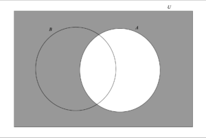
Venn diagrams use overlapping circles inside a rectangle (the sample space) to represent events.
- The rectangle represents the whole sample space U.
- Each circle represents an event (e.g. A, B, C).
- The overlap A ∩ B shows outcomes where both events occur.
- The outer parts of each circle show outcomes where only that event occurs.
- The area outside all circles represents outcomes where none of the events occur
Tree diagrams
Tree diagrams display multi-stage experiments step by step.
- Each branch is labelled with the probability of that outcome at that stage.
- Probabilities along a path are multiplied to find the probability of that combined outcome.
- Probabilities of different paths are added when representing “or” situations.
- Tree diagrams are very helpful for problems with or without replacement.
🧠 Examiner Tip:
For multi-step questions, you will often earn method marks simply for drawing a correct tree diagram
with probabilities on the branches. Even if an arithmetic mistake occurs later, the diagram can protect marks.
🌍 Real-World Connection:
Tree-like models are used in decision analysis, where each branch represents a decision or chance outcome
(for example, market up/down, drug effective/ineffective). Probabilities along branches help estimate expected profits or risks.
2. Combined Events – “A or B”
General addition rule
For any two events A and B:
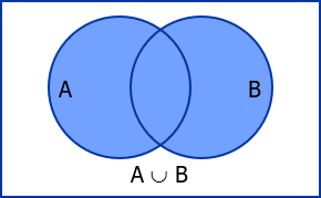
P(A ∪ B) = P(A) + P(B) − P(A ∩ B)
- A ∪ B means “A or B or both”.
- The term P(A ∩ B) is subtracted because the overlap has been counted twice: once in P(A) and once in P(B).
- This rule expresses the non-exclusivity of “or” in probability.
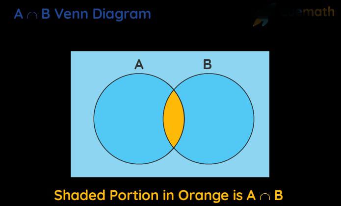
Intersection of Events (A ∩ B)
The intersection of two events A and B, written as A ∩ B, represents all outcomes that belong to both A and B at the same time.
Graphically, it is shown as the overlapping region in a Venn diagram.
Probabilistically, P(A ∩ B) measures the chance of A and B occurring together.
When A and B have no overlap, their intersection is empty and P(A ∩ B) = 0, meaning they are mutually exclusive.
Mutually exclusive events
- Events A and B are mutually exclusive if they cannot happen at the same time: P(A ∩ B) = 0.
- For mutually exclusive events, the rule simplifies to: P(A ∪ B) = P(A) + P(B).
- On a Venn diagram, mutually exclusive events have no overlap.
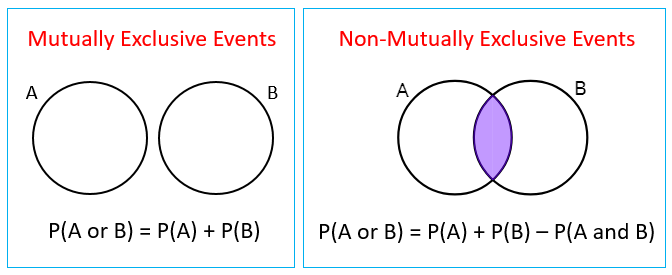
https://www.onlinemathlearning.com/image-files/probability-mutually-exclusive.png
Example (combined events):
In a survey, 60% of students like coffee (A) and 40% like tea (B). If 25% like both coffee and tea,
P(A ∪ B) = 0.60 + 0.40 − 0.25 = 0.75 → 75% like at least one of the two.
📝 Paper 1 Strategy:
When you see the word “or” in a probability question, pause and check:
Can both events happen together?
If yes, use the full formula with −P(A ∩ B); if no, simply add P(A) and P(B).
3. Conditional Probability – P(A|B)
Definition and meaning
- Conditional probability describes the chance of event A occurring given that event B has already happened.
- It “shrinks” the sample space to only those outcomes where B is true.
- Formula: P(A|B) = P(A ∩ B) / P(B), provided P(B) ≠ 0.
Rearranging gives another useful form:
P(A ∩ B) = P(B) P(A|B)
This version often appears in tree diagrams: the joint probability of A and B is the probability of reaching B,
multiplied by the conditional probability of A at that stage.
Example – card drawing (without replacement)
Two cards are drawn in order from a standard 52-card deck, without replacement.
Let A = “second card is a heart”, B = “first card is a heart”.
- P(B) = 13/52 = 1/4.
- If B has happened, there are now 12 hearts left out of 51 cards → P(A|B) = 12/51.
- P(A ∩ B) = P(B)P(A|B) = (1/4) × (12/51) = 12/204 = 1/17.
💻 GDC Use:
For complex conditional probability questions, especially with many branches, you can verify results
using a GDC’s table or simulation functions. However, in Paper 1 you must still show
the algebra or tree diagram to earn full method marks.
🧠 Examiner Tip:
Many students confuse P(A|B) with P(B|A). In the exam, write a short sentence such as
“P(A|B) = probability that A happens given B has occurred” before using the formula.
This helps you choose the correct conditional direction.
4. Independent Events – No Influence
Definition
- Events A and B are independent if the occurrence of one does not affect the probability of the other.
- Formally, A and B are independent if P(A|B) = P(A) (and equivalently P(B|A) = P(B)).
- This leads to: P(A ∩ B) = P(A)P(B).
Example: Tossing a fair coin and rolling a fair die.
A = “coin shows heads”, B = “die shows 6”.
P(A) = 1/2, P(B) = 1/6, and P(A ∩ B) = 1/12 = (1/2) × (1/6), so A and B are independent.
📝 Paper 2 Tip:
When a question gives you P(A), P(B) and P(A ∩ B), quickly test whether
P(A ∩ B) equals P(A)P(B). If yes, state clearly that A and B are independent and use this result
to simplify later calculations.
5. With and Without Replacement
Many conditional probability problems involve whether items are replaced after each draw.
- With replacement: after each selection, the object is returned.
Probabilities stay the same for each draw → often leads to independent events.
- Without replacement: objects are not returned.
Probabilities change after each draw → events are usually dependent.
- Tree diagrams clearly show how branch probabilities alter when there is no replacement.
🔍 TOK / Ethics Connection:
Probability models are used in gambling, lotteries and online gaming.
How should mathematicians and game designers consider the ethics of using sophisticated probability
calculations to design games where the house has a long-term advantage?
Should mathematics be used to maximise profit from players who may not understand these models?
Mastering SL 4.6 means being comfortable switching between diagrams, formulas and contextual reasoning.
Always check whether events overlap, are conditional on each other, or are independent, and then choose the
appropriate probability rule.