This question bank contains 11 questions covering partial fraction decomposition techniques, including linear factors, repeated factors, and quadratic factors, distributed across different paper types according to IB AAHL curriculum standards.
📌 Multiple Choice Questions (2 Questions)
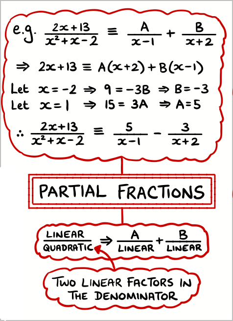
MCQ 1. The partial fraction decomposition of \(\frac{3x+2}{(x-1)(x+3)}\) is:
A) \(\frac{5/4}{x-1} + \frac{7/4}{x+3}\) B) \(\frac{7/4}{x-1} + \frac{5/4}{x+3}\) C) \(\frac{5/4}{x-1} – \frac{7/4}{x+3}\) D) \(\frac{-1/4}{x-1} + \frac{11/4}{x+3}\)
📖 Show Answer
Solution:
Set up: \(\frac{3x+2}{(x-1)(x+3)} = \frac{A}{x-1} + \frac{B}{x+3}\)
Clear denominators: \(3x+2 = A(x+3) + B(x-1)\)
x = 1: 3(1)+2 = A(4) → 5 = 4A → A = 5/4
x = -3: 3(-3)+2 = B(-4) → -7 = -4B → B = 7/4
✅ Answer: A) \(\frac{5/4}{x-1} + \frac{7/4}{x+3}\)
MCQ 2. Which setup is correct for \(\frac{2x^2+x+1}{x(x-1)^2}\)?
A) \(\frac{A}{x} + \frac{B}{(x-1)^2}\) B) \(\frac{A}{x} + \frac{B}{x-1} + \frac{C}{(x-1)^2}\) C) \(\frac{Ax+B}{x(x-1)^2}\) D) \(\frac{A}{x} + \frac{Bx+C}{(x-1)^2}\)
📖 Show Answer
Solution:
For simple linear factor x, we need \(\frac{A}{x}\)
For repeated linear factor (x-1)², we need both \(\frac{B}{x-1}\) and \(\frac{C}{(x-1)^2}\)
Paper 2 – Q4. A rational function has the form \(\frac{ax+b}{(x-1)(x+2)}\). If the partial fraction decomposition is \(\frac{2}{x-1} + \frac{3}{x+2}\), find the values of a and b.
Preparation for integration techniques in calculus.
Link to polynomial long division when degree of numerator ≥ degree of denominator.
Method of undetermined coefficients.
Cover-up method for simple linear factors.
Applications in differential equations and Laplace transforms.
Connection to complex numbers and residue theory.
Use of technology for verification and complex cases.
📌 Introduction
Partial fraction decomposition represents one of the most elegant and powerful techniques in algebraic manipulation, serving as a crucial bridge between rational function theory and advanced calculus. This sophisticated method transforms complex rational expressions into simpler, more manageable components, enabling mathematicians to tackle integration problems that would otherwise be intractable. The technique’s fundamental principle—breaking down a complicated fraction into a sum of simpler fractions—mirrors the mathematical philosophy of divide and conquer that underlies much of advanced mathematics.
The historical development of partial fractions traces back to the work of Leibniz and the Bernoulli brothers, who recognized that rational functions could be systematically decomposed into elementary components. This decomposition not only simplifies algebraic manipulation but also reveals the underlying structure of rational expressions, connecting abstract algebra with practical applications in physics, engineering, and advanced mathematics. From solving differential equations to analyzing electrical circuits, partial fractions provide the mathematical foundation for understanding complex systems through the lens of simpler, constituent parts.
📌 Definition Table
Term
Definition
Partial Fraction
A fraction with a simpler denominator that forms part of a partial fraction decomposition
Example: \(\frac{A}{x-1}\) or \(\frac{Bx+C}{x^2+1}\)
Partial Fraction Decomposition
The process of expressing a rational function as a sum of simpler partial fractions
\(\frac{P(x)}{Q(x)} = \frac{A_1}{(x-r_1)} + \frac{A_2}{(x-r_2)} + \cdots\)
Proper Rational Function
A rational function where degree of numerator < degree of denominator
Required for direct partial fraction decomposition
Improper Rational Function
A rational function where degree of numerator ≥ degree of denominator
Requires polynomial long division before partial fraction decomposition
Linear Factor
A factor of the form (x – a) or (ax + b)
Contributes \(\frac{A}{x-a}\) to the decomposition
Repeated Linear Factor
A factor of the form (x – a)ⁿ where n > 1
Contributes \(\frac{A_1}{x-a} + \frac{A_2}{(x-a)^2} + \cdots + \frac{A_n}{(x-a)^n}\)
Quadratic Factor
An irreducible factor of the form ax² + bx + c (no real roots)
Contributes \(\frac{Bx+C}{ax^2+bx+c}\) to the decomposition
Cover-up Method
A shortcut technique for finding coefficients of simple linear factors
“Cover up” the factor and substitute its root
📌 Properties & Key Formulas
Basic Decomposition Types:
Linear factors: \(\frac{P(x)}{(x-a)(x-b)} = \frac{A}{x-a} + \frac{B}{x-b}\)
How to avoid: Quadratic factors require linear numerators (Ax + B).
⚠️ Common Mistake #4: Arithmetic errors in coefficient finding
Wrong: Making sign errors when substituting values or equating coefficients Right: Systematically check each step, especially with negative substitutions
How to avoid: Use multiple methods to verify coefficients and always check final answer.
⚠️ Common Mistake #5: Incomplete factorization of denominator
How to avoid: Always factor denominators completely before setting up partial fractions.
📌 Calculator Skills: Casio CG-50 & TI-84
📱 Using Casio CG-50 for Partial Fractions
Polynomial Long Division:
1. [MENU] → “Algebra” → “Polynomial Tools”
2. Select “Divide” for polynomial division
3. Enter numerator and denominator polynomials
4. Get quotient and remainder automatically
Verification of Results:
1. Use “expand” to combine partial fractions
2. Store original expression in one variable
3. Store partial fraction sum in another
4. Subtract to verify they’re equal (should be 0)
Solving Systems for Coefficients:
1. [MENU] → “Equation/Inequality” → “Solver”
2. Set up system of equations from coefficient equating
3. Solve for unknown coefficients simultaneously
4. Use substitution method for verification
📱 Using TI-84 for Partial Fractions
Basic Factoring:
1. Use “factor(” command for polynomial factoring
2. Example: factor(x^3-6x^2+11x-6)
3. Verify results by expanding back
4. Check degree and leading coefficient
Polynomial Division:
1. Manual long division using paper method
2. Verify using polynomial evaluation at test points
3. Use [MATH] → [0:solve(] for finding roots
4. Build factors from known roots
System Solving:
1. Use matrix operations for coefficient systems
2. [2nd] [MATRIX] → “MATH” → “rref(“
3. Set up augmented matrix for coefficients
4. Solve using reduced row echelon form
Verification Techniques:
1. Define original function as Y1
2. Define partial fraction sum as Y2
3. Graph Y1-Y2 to check for zero difference
4. Use [2nd] [TRACE] → “value” for spot checks
📱 Advanced Problem-Solving Techniques
Complex Factorization:
• Use numerical methods to find approximate roots
• Apply synthetic division for known factors
• Check discriminant for quadratic factors
• Use graphing to identify multiplicity of roots
Coefficient Verification:
• Test multiple x-values in original vs. decomposition
• Use specific values like x = 0, 1, -1 for quick checks
• Verify degree consistency throughout process
• Check limiting behavior as x approaches infinity
Error Prevention:
• Save intermediate results to avoid recomputation
• Use parentheses carefully in complex expressions
• Double-check signs when working with negative roots
• Maintain fraction forms when possible for exact answers
📌 Mind Map
📌 Applications in Science and IB Math
Calculus Integration: Essential for integrating rational functions, fundamental theorem applications
Differential Equations: Solution techniques, Laplace transforms, system analysis
Engineering: Circuit analysis, signal processing, control systems design
Statistics: Probability generating functions, moment calculations, distribution analysis
Pure Mathematics: Complex analysis, algebraic number theory, abstract algebra
➗ IA Tips & Guidance:Partial fractions provide excellent opportunities for connecting algebraic techniques with advanced mathematical applications across multiple disciplines.
Excellent IA Topics:
• Historical development of partial fraction techniques and mathematical contributions
• Engineering applications: RC circuits and impedance analysis using partial fractions
• Economics modeling: cost functions and marginal analysis with rational expressions
• Population dynamics: differential equation solutions via partial fraction methods
• Signal processing: Fourier analysis and frequency domain techniques
• Probability theory: moment generating functions and distribution decomposition
• Numerical analysis: integration algorithms and computational efficiency
• Music theory: harmonic analysis and acoustic wave decomposition
IA Structure Tips:
• Begin with historical context and motivation for the technique
• Develop theoretical foundations systematically
• Include substantial real-world applications with actual data
• Connect to other mathematical areas (calculus, differential equations)
• Explore computational aspects and algorithm efficiency
• Use technology to handle complex cases and verify results
• Discuss limitations and extensions to advanced mathematics
• Include original research or novel applications
• Address both theoretical beauty and practical utility
📌 Worked Examples (IB Style)
Q1. Express \(\frac{7x+1}{(x-1)(x+2)}\) in partial fractions.
Solution:
Step 1: Set up partial fraction form
\(\frac{7x+1}{(x-1)(x+2)} = \frac{A}{x-1} + \frac{B}{x+2}\)
Step 3: Find coefficients using substitution
x = 1: \(3(1)^2+2(1)+1 = B(1+1) \Rightarrow 6 = 2B \Rightarrow B = 3\)
x = -1: \(3(-1)^2+2(-1)+1 = C(-1-1)^2 \Rightarrow 2 = 4C \Rightarrow C = \frac{1}{2}\)
Step 4: Find A by equating coefficients
Expanding: \(3x^2+2x+1 = A(x^2-1) + B(x+1) + C(x-1)^2\)
Coefficient of x²: 3 = A + C = A + \frac{1}{2} \Rightarrow A = \frac{5}{2}\)
Step 4: Expand and equate coefficients
\(2x^3-x^2+x-1 = Ax^3+Ax+Bx^2+B+Cx+D\)
x³: 2 = A ⇒ A = 2
x²: -1 = B ⇒ B = -1
x¹: 1 = A + C = 2 + C ⇒ C = -1
x⁰: -1 = B + D = -1 + D ⇒ D = 0
📝 Paper Tip:For AHL partial fraction problems, always show your method clearly: factorization, setup, coefficient determination, and verification.
Key strategies for success:
• Check degree first – divide if improper
• Factor completely before setting up
• Use cover-up method for simple linear factors
• Set up systematic equations for complex cases
• Always verify by combining back to original
• Show all algebraic steps clearly
This question bank contains 22 questions covering advanced counting principles, permutations, combinations, and sophisticated combinatorial problems, distributed across different paper types according to IB AAHL curriculum standards.
📌 Multiple Choice Questions (4 Questions)
MCQ 1. In how many ways can 6 people be arranged in a circle?
A) 6! B) 5! C) (6-1)! D) 6!/6
📖 Show Answer
Solution:
For circular permutations, we fix one person to eliminate rotational symmetry.
With n people in a circle, there are (n-1)! arrangements.
For 6 people: (6-1)! = 5! = 120 ways
✅ Answer: C) (6-1)!
MCQ 2. How many different arrangements can be made from the letters of the word “COMMITTEE”?
A) 7560 B) 45360 C) 181440 D) 362880
📖 Show Answer
Solution:
COMMITTEE has 9 letters: C(1), O(1), M(2), I(1), T(2), E(2)
✅ Answers:
(i) 175,760,000 passwords
(ii) 78,624,000 passwords
Paper 2 – Q2. A quality control inspector selects 5 items from a batch of 20 items (12 good, 8 defective). Find the probability that exactly 2 items are defective.
[5 marks]
📖 Show Answer
Solution:
Step 1: Identify the scenario
Need exactly 2 defective and 3 good items
Step 2: Count favorable outcomes
Ways to choose 2 defective from 8: \({}^8C_2 = \frac{8 \times 7}{2} = 28\)
Ways to choose 3 good from 12: \({}^{12}C_3 = \frac{12 \times 11 \times 10}{6} = 220\)
Favorable outcomes = \(28 \times 220 = 6160\)
Step 3: Count total outcomes
Total ways to choose 5 from 20: \({}^{20}C_5 = 15504\)
Step 4: Calculate probability
Probability = \(\frac{6160}{15504} = \frac{385}{969} ≈ 0.397\)
✅ Answer: \(\frac{385}{969}\) or approximately 0.397
Paper 2 – Q3. In a tournament, 16 teams play in a knockout format. How many different ways can the tournament brackets be arranged for the first round if teams are grouped into 4 groups of 4 teams each?
[6 marks]
📖 Show Answer
Solution:
Step 1: Understand the grouping
16 teams divided into 4 groups of 4 teams each
Groups are distinguishable (Group A, B, C, D)
Step 2: Calculate step by step
Group A: Choose 4 from 16 teams: \({}^{16}C_4 = 1820\)
Group B: Choose 4 from remaining 12: \({}^{12}C_4 = 495\)
Group C: Choose 4 from remaining 8: \({}^8C_4 = 70\)
✅ Final Answers:
(a) 0.309
(b) 3360 ways
(c) A only: 200, B only: 300, Both: 100, Neither: 400
Paper 3 – Q3. A computer programmer is designing secure passwords. The password must contain exactly 8 characters with specific requirements.
(a) How many 8-character passwords can be formed using 26 letters and 10 digits if each password must contain at least one digit and at least one letter? [4 marks]
(b) If the password must also contain at least one uppercase letter, one lowercase letter, and one special character from a set of 8 symbols, how many passwords are possible? [6 marks]
(c) Compare the security strength of passwords from parts (a) and (b) by calculating the ratio. [2 marks]
\({}^nP_r = \frac{n!}{(n-r)!}\) and \({}^nC_r = \binom{n}{r} = \frac{n!}{r!(n-r)!}\)
Arrangements with restrictions.
Circular permutations.
Applications to probability.
Link to SL 1.9 Binomial theorem.
Use of technology to calculate large factorials.
Distinguishing between situations requiring permutations vs combinations.
Advanced topics: arrangements with identical objects, conditional arrangements, inclusion-exclusion principle.
Applications in genetics, computer science, and quality control.
Link to binomial and multinomial distributions in statistics.
Extension to probability spaces and sample counting.
📌 Introduction
Combinatorics, the mathematics of counting, stands as one of the most fundamental yet sophisticated branches of discrete mathematics. From ancient problems like determining the number of ways to arrange objects to modern applications in cryptography, computer science, and probability theory, counting principles provide the essential tools for analyzing complex systems where order, selection, and arrangement matter. The elegance of combinatorial thinking lies in its ability to transform seemingly impossible counting problems into systematic, calculable solutions.
This advanced topic builds directly on the binomial theorem from SL 1.9, revealing the deep connections between algebraic expansion and combinatorial selection. The fundamental counting principle forms the cornerstone, while permutations and combinations provide specialized tools for handling ordered and unordered selections respectively. As we progress to arrangements with restrictions, circular permutations, and real-world applications, we discover that combinatorics is not just about counting—it’s about understanding the structure and possibilities inherent in mathematical systems, making it indispensable for advanced probability, statistics, and theoretical computer science.
📌 Definition Table
Term
Definition
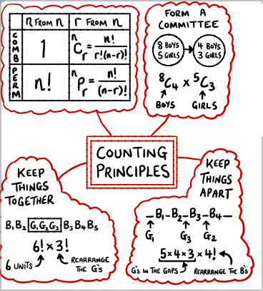
Fundamental Counting Principle
If task A can be done in m ways and task B in n ways,
then both tasks can be done in m × n ways
Factorial
\(n! = n \times (n-1) \times (n-2) \times \cdots \times 2 \times 1\)
By convention: \(0! = 1\)
Permutation
An arrangement of objects where order matters
\({}^nP_r = \frac{n!}{(n-r)!}\) ways to arrange r objects from n objects
Combination
A selection of objects where order does not matter
\({}^nC_r = \binom{n}{r} = \frac{n!}{r!(n-r)!}\) ways to choose r objects from n objects
Circular Permutation
Arrangement of objects in a circle
\((n-1)!\) ways to arrange n distinct objects in a circle
Restricted Arrangement
Permutations with constraints (objects together, apart, or in specific positions)
Requires systematic case-by-case analysis
Repeated Objects
Arrangements of n objects with repeated elements
\(\frac{n!}{n_1! \times n_2! \times \cdots \times n_k!}\) for k types of repeated objects
Step 1: Is order important?
YES → Use Permutations
NO → Use Combinations
Step 2: Are there restrictions?
YES → Use complementary counting or case analysis
NO → Apply direct formula
Step 3: Are objects identical?
YES → Use multinomial coefficients
NO → Use standard formulas
Step 4: Circular arrangement?
YES → Use (n-1)! formula
NO → Use standard permutation formula
Advanced Counting Scenarios:
Committee Selection: Use combinations \({}^nC_r\)
Password Creation: Use permutations with repetition
Seating Arrangements: Use permutations or circular permutations
Distribution Problems: Use multinomial coefficients
Tournament Brackets: Systematic counting with restrictions
Graph Theory: Counting paths, trees, and matchings
🧠 Examiner Tip:Always ask yourself: “Does order matter?” This single question determines whether to use permutations or combinations.
Remember: Permutations for arrangements (line up people), combinations for selections (choose team members).
📌 Common Mistakes & How to Avoid Them
⚠️ Common Mistake #1: Confusing permutations and combinations
Wrong: “Choose 3 people from 10 for a team” using \({}^{10}P_3\) Right: Use \({}^{10}C_3\) because order doesn’t matter in team selection
How to avoid: Ask “If I swap two selected items, is it a different outcome?”
⚠️ Common Mistake #2: Incorrect handling of restrictions
Wrong: “Arrange 5 people with 2 specific people together” by treating as 4 objects Right: Treat the 2 people as one unit (4! arrangements) × internal arrangements (2!) = 4! × 2!
How to avoid: Use systematic case analysis or complementary counting.
⚠️ Common Mistake #3: Forgetting to account for identical objects
Wrong: Arranging letters in “MATHEMATICS” using 11! Right: \(\frac{11!}{2! \times 2! \times 2!}\) (accounting for repeated M, A, T)
How to avoid: Always identify and count repeated elements before calculating.
⚠️ Common Mistake #4: Circular permutation errors
Wrong: Seating 6 people around a circular table using 6! Right: Use (6-1)! = 5! because circular arrangements eliminate one degree of freedom
How to avoid: Remember that in circles, rotations are considered identical.
⚠️ Common Mistake #5: Double counting in complex problems
Wrong: Counting arrangements and then forgetting some cases overlap Right: Use inclusion-exclusion principle or carefully define mutually exclusive cases
How to avoid: Clearly define what makes two outcomes different before counting.
📌 Calculator Skills: Casio CG-50 & TI-84
📱 Using Casio CG-50 for Counting & Combinatorics
Factorial Calculations:
1. Input number, then [OPTN] → [PROB] → [x!]
2. Example: 8[x!] gives 40320
3. For large factorials: Use scientific notation display
Advanced Calculations:
1. Use [MENU] → “Statistics” for probability distributions
2. Store values in variables for complex calculations
3. Use parentheses for multi-step calculations
Basic Operations:
1. [MATH] → [PRB] → [4:!] for factorials
2. [MATH] → [PRB] → [2:nPr] for permutations
3. [MATH] → [PRB] → [3:nCr] for combinations
Complex Calculations:
1. Use [STO] to store intermediate results
2. Example: 8[!]/((8-3)[!]) for P(8,3)
3. Use [ANS] to build on previous calculations
Programming for Repetitive Tasks:
1. [PRGM] → [NEW] to create programs
2. Useful for multinomial coefficients
3. Can automate restriction-based counting
Statistical Applications:
1. [2nd] [DISTR] for probability distributions
2. Link combinatorics to binomial probabilities
3. Use for Monte Carlo simulations
📱 Advanced Problem-Solving Techniques
Large Number Handling:
• Use logarithms for very large factorials
• Simplify fractions before calculating
• Check for common factors in numerator/denominator
Verification Methods:
• Small case testing: verify formulas with n=3,4,5
• Symmetry checks: C(n,r) should equal C(n,n-r)
• Boundary testing: check n=r and r=0 cases
Problem-solving workflow:
• Identify the counting type (permutation/combination)
• Check for restrictions or special conditions
• Calculate step by step, storing intermediate values
• Verify answer using alternative methods when possible
📌 Mind Map
📌 Applications in Science and IB Math
Computer Science: Algorithm complexity analysis, cryptography, data structures
Genetics: DNA sequence analysis, inheritance patterns, population genetics
Biology: Ecological modeling, species distribution, evolutionary pathways
Pure Mathematics: Graph theory, number theory, algebraic structures
➗ IA Tips & Guidance:Combinatorics offers rich opportunities for exploring both theoretical mathematics and practical applications across multiple disciplines.
Excellent IA Topics:
• Genetic inheritance modeling using advanced combinatorial techniques
• Cryptographic analysis: combinations in code-breaking and security
• Sports tournament design and optimization using combinatorial principles
• Social network analysis: counting connections and influence patterns
• Card game mathematics: probability and counting in poker, bridge
• DNA sequence analysis: combinatorial approaches to genetic patterns
• Traffic flow optimization: combinations in urban planning
• Art and design: combinatorial aesthetics and pattern generation
IA Structure Tips:
• Begin with simple, concrete examples before advancing to complex theory
• Use technology to verify calculations and explore large-scale patterns
• Include historical development and multiple cultural perspectives
• Connect theoretical results to real-world data and applications
• Explore extensions like generating functions or recurrence relations
• Use statistical analysis to validate combinatorial models
• Create visual representations of complex counting scenarios
• Discuss computational complexity and algorithmic approaches
• Address limitations and assumptions in real-world modeling
📌 Worked Examples (IB Style)
Q1. In how many ways can 7 people be arranged in a line if 2 specific people must not stand next to each other?
Solution:
Method: Complementary counting
Total arrangements – Arrangements with 2 people together
Step 1: Total arrangements of 7 people
Total = 7! = 5040
Step 2: Arrangements with 2 specific people together
Treat the 2 people as one unit → 6 units to arrange
Arrangements = 6! × 2! = 720 × 2 = 1440
(6! for arranging units, 2! for internal arrangement)
Q2. A committee of 5 people is to be selected from 8 men and 6 women. Find the number of ways if the committee must have at least 2 women.
Solution:
Method: Case-by-case analysis
Case 1: Exactly 2 women, 3 men
Ways = \({}^6C_2 \times {}^8C_3 = 15 \times 56 = 840\)
Case 2: Exactly 3 women, 2 men
Ways = \({}^6C_3 \times {}^8C_2 = 20 \times 28 = 560\)
Case 3: Exactly 4 women, 1 man
Ways = \({}^6C_4 \times {}^8C_1 = 15 \times 8 = 120\)
Case 4: Exactly 5 women, 0 men
Ways = \({}^6C_5 \times {}^8C_0 = 6 \times 1 = 6\)
Total: 840 + 560 + 120 + 6 = 1526
✅ Answer: 1526 ways
Q3. In how many ways can the letters of the word “STATISTICS” be arranged?
Solution:
Step 1: Count letters and repetitions
STATISTICS has 10 letters:
S appears 3 times, T appears 3 times, A appears 1 time,
I appears 2 times, C appears 1 time
Step 2: Apply formula for repeated objects
\(\text{Arrangements} = \frac{n!}{n_1! \times n_2! \times \cdots \times n_k!}\)
Q4. Find the number of ways 8 people can be seated around a circular table if 2 specific people must sit together.
Solution:
Step 1: Treat the 2 specific people as one unit
We now have 7 units to arrange in a circle
Step 2: Arrange units in a circle
Number of ways = (7-1)! = 6! = 720
Step 3: Account for internal arrangement
The 2 specific people can be arranged in 2! = 2 ways
Step 4: Calculate total
Total arrangements = 6! × 2! = 720 × 2 = 1440
✅ Answer: 1440 ways
Q5. A password consists of 4 digits followed by 3 letters. How many different passwords are possible if repetition is allowed?
Solution:
Step 1: Apply fundamental counting principle
Total possibilities = (choices for digits) × (choices for letters)
Step 2: Count digit possibilities
4 digit positions, each can be 0-9 (10 choices)
With repetition allowed: \(10^4 = 10,000\) possibilities
Step 3: Count letter possibilities
3 letter positions, each can be A-Z (26 choices)
With repetition allowed: \(26^3 = 17,576\) possibilities
Step 4: Calculate total passwords
Total = \(10^4 \times 26^3 = 10,000 \times 17,576 = 175,760,000\)
✅ Answer: 175,760,000 passwords
📝 Paper Tip:For AHL counting problems, always clearly state your strategy (direct counting, complementary counting, or case analysis) before beginning calculations.
Key problem-solving strategies:
• Identify whether order matters (permutation vs combination)
• Look for restrictions and handle them systematically
• Use complementary counting for “at least” or “at most” problems
• Break complex problems into simpler cases
• Always verify your answer makes intuitive sense
• Check boundary cases and special conditions
This question bank contains 17 questions covering the binomial theorem, binomial coefficients, and expansion techniques, distributed across different paper types according to IB AAHL curriculum standards.
📌 Multiple Choice Questions (3 Questions)
MCQ 1. What is the coefficient of \(x^5\) in the expansion of \((x + 2)^8\)?
A) 56 B) 112 C) 224 D) 448
📖 Show Answer
Solution:
General term: \(T_{r+1} = \binom{8}{r} x^{8-r} 2^r\)
Using symmetry property: \(\binom{n}{r} = \binom{n}{n-r}\)
\(\binom{7}{5} = \binom{7}{7-5} = \binom{7}{2}\)
Therefore, coefficient of \(x^5\) = coefficient of \(x^2\) = 21
✅ Final Answers:
(a) \(1 + nx + \frac{n(n-1)}{2}x^2 + \frac{n(n-1)(n-2)}{6}x^3\)
(b) n = 7
(c) 21
(d) Proven by symmetry property
Paper 3 – Q2. A biologist is studying genetic inheritance. In a certain species, offspring inherit two alleles for a trait, one from each parent. Each parent passes on allele A with probability 0.6 and allele a with probability 0.4.
(a) Use the binomial theorem to find the probability distribution for the number of A alleles in an offspring. [3 marks]
(b) What is the probability an offspring has exactly one A allele? [2 marks]
(c) If the biologist examines 5 offspring, what is the expected number with genotype Aa? [3 marks]
(d) Expand \((0.6 + 0.4)^{10}\) and interpret this result biologically. [4 marks]
📖 Show Answer
Complete solution:
(a) Probability distribution:
Using \((p + q)^n\) where p = 0.6 (prob of A), q = 0.4 (prob of a), n = 2
Sum formula: \(2^0 = 1\) (correct, since row 0 has only entry 1)
Alternating formula: \(0^0 = 1\) (by convention)
Significance: Both give the same result (1) for the base case,
showing the consistency of the mathematical definitions.
✅ Final Answers:
(a) 1, 6, 15, 20, 15, 6, 1
(b) Sum = \(2^n\)
(c) Alternating sum = \(0^n\)
(d) 64 and 0 respectively
(e) Both equal 1, showing base case consistency
Paper 3 – Q4. A company is developing a new product. The probability of success at each stage of development is 0.8, and there are n independent stages.
(a) Write an expression for the probability of exactly k successes. [2 marks]
(b) If n = 5, find the probability of exactly 4 successes. [3 marks]
(c) For n = 5, what is the most likely number of successes? Justify your answer. [4 marks]
(d) The company needs at least 4 successes out of 5 stages. Calculate this probability and comment on the viability. [3 marks]
📖 Show Answer
Complete solution:
(a) General probability expression:
Using binomial probability:
\(P(X = k) = \binom{n}{k} (0.8)^k (0.2)^{n-k}\)
(b) Probability of exactly 4 successes when n = 5:
Expansion of \((a+b)^n\) where n is a positive integer.
Binomial coefficients.
\(\binom{n}{r} = {}^nC_r = \frac{n!}{r!(n-r)!}\)
The general term.
Link to 1.1 Operations with numbers.
Pascal’s triangle and its properties.
Use of technology to calculate binomial coefficients.
Link to AHL 1.10 for more advanced counting principles.
Applications in probability and statistics.
The general term is \(T_{r+1} = \binom{n}{r} a^{n-r} b^r\).
📌 Introduction
The binomial theorem is one of the most elegant and powerful results in algebra, providing a systematic way to expand expressions of the form (a + b)ⁿ where n is a positive integer. Named after the Latin word “binomium” meaning “two terms,” this theorem transforms what would be tedious multiplication into a precise formula involving binomial coefficients. The theorem’s applications extend far beyond simple algebraic manipulation, forming the foundation for probability theory, combinatorics, and advanced mathematical analysis.
The beauty of the binomial theorem lies in its connection to Pascal’s triangle, where each row provides the coefficients for the expansion. This visual representation reveals deep patterns and relationships that have fascinated mathematicians for centuries. From calculating compound interest to determining probabilities in genetics, the binomial theorem provides both computational tools and theoretical insights that bridge pure mathematics with real-world applications across science, economics, and technology.
📌 Definition Table
Term
Definition
Binomial Expression
An algebraic expression with exactly two terms
Example: (a + b), (x – 2), (3m + 5n)
Binomial Theorem
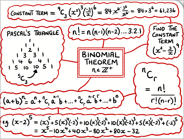
\((a+b)^n = \sum_{r=0}^{n} \binom{n}{r} a^{n-r} b^r\)
Systematic method to expand binomial expressions raised to positive integer powers
Binomial Coefficient
\(\binom{n}{r} = {}^nC_r = \frac{n!}{r!(n-r)!}\)
The coefficient of the (r+1)th term in the expansion of (a+b)ⁿ
Factorial
\(n! = n \times (n-1) \times (n-2) \times \cdots \times 2 \times 1\)
By convention: 0! = 1
General Term
\(T_{r+1} = \binom{n}{r} a^{n-r} b^r\)
The (r+1)th term in the expansion of (a+b)ⁿ
Pascal’s Triangle
A triangular array where each number is the sum of the two above it
Each row n gives the binomial coefficients for (a+b)ⁿ
Combinatorial Notation
\(\binom{n}{r}\) read as “n choose r”
Represents the number of ways to choose r objects from n objects
Symmetric Property
\(\binom{n}{r} = \binom{n}{n-r}\)
Binomial coefficients are symmetric about the middle
How to avoid: Double-check factorial calculations and use calculator when allowed.
⚠️ Common Mistake #4: Forgetting the coefficient in the general term
Wrong: For \((2x+3)^5\), writing the general term as \(\binom{5}{r} (2x)^{5-r} 3^r\) Right: General term is \(\binom{5}{r} (2x)^{5-r} 3^r = \binom{5}{r} 2^{5-r} 3^r x^{5-r}\)
How to avoid: Always expand numerical coefficients like \((2x)^{5-r} = 2^{5-r}x^{5-r}\).
⚠️ Common Mistake #5: Misidentifying middle terms
Wrong: For \((a+b)^6\), claiming the middle term is the 3rd term Right: For \((a+b)^6\) (7 terms total), the middle term is the 4th term: \(T_4 = \binom{6}{3} a^3 b^3\)
How to avoid: Count carefully: for n even, there’s one middle term; for n odd, two middle terms.
Factorial Calculations:
1. Input number, then [OPTN] → [PROB] → [x!]
2. Example: 5[x!] gives 120
3. For verification: 8[x!] ÷ (3[x!] × 5[x!]) should equal \(\binom{8}{3}\)
Polynomial Expansion:
1. Use [MENU] → “Algebra” → “Polynomial Tools”
2. Enter expression like (x+2)^4
3. Select “Expand” to get full expansion
Finding Specific Terms:
1. Store values: a, b, n, r in variables
2. Calculate: [nCr](n,r) × a^(n-r) × b^r
3. Substitute numerical values to get final answer
Expansion Verification:
1. [Y=] → Enter (x+2)^4 as Y1
2. [Y=] → Enter expanded form as Y2
3. [GRAPH] → Both should be identical
Polynomial Tools:
1. Use [APPS] → [PolySmlt2] for polynomial operations
2. Can handle symbolic expansions
3. Useful for verifying manual calculations
📱 Advanced Calculator Techniques
Pattern Recognition:
• Generate Pascal’s triangle rows using combinations
• Verify symmetry: \(\binom{n}{r} = \binom{n}{n-r}\)
• Check sum property: sum of row n should equal 2ⁿ
Error Prevention:
• Always verify binomial coefficients with factorial formula
• Use parentheses carefully in complex expressions
• Double-check sign patterns in alternating expansions
Problem-solving shortcuts:
• Store common values (n, a, b) in calculator memory
• Use ANS function to build calculations step by step
• Create simple programs for repetitive calculations
📌 Mind Map
📌 Applications in Science and IB Math
Probability Theory: Binomial distribution, coin flips, quality control sampling
Physics: Quantum mechanics probability amplitudes, statistical mechanics
Engineering: Signal processing, error correction codes, network reliability
Biology: Genetics inheritance patterns, population dynamics, evolutionary models
Chemistry: Molecular orbital theory, reaction pathway analysis
Pure Mathematics: Combinatorics, number theory, algebraic topology
➗ IA Tips & Guidance:The binomial theorem offers rich opportunities for exploring connections between algebra, combinatorics, and real-world applications.
Excellent IA Topics:
• Pascal’s triangle patterns and their mathematical significance
• Binomial distribution applications in quality control or medical testing
• Mathematical analysis of genetic inheritance using binomial probabilities
• Financial modeling: portfolio risk using binomial trees
• Sports analytics: predicting outcomes using binomial models
• Computer algorithms: error detection and correction using binomial coefficients
• Historical mathematics: development of binomial theorem across cultures
• Approximation techniques: using binomial theorem for near-integer powers
IA Structure Tips:
• Start with concrete examples before introducing general formulas
• Use technology to verify patterns and generate large-scale data
• Include historical context and multiple mathematical perspectives
• Connect theoretical results to practical applications
• Explore extensions like multinomial theorem or negative exponents
• Use statistical analysis to validate probabilistic applications
• Create visual representations of Pascal’s triangle patterns
• Discuss limitations and assumptions in real-world modeling
📌 Worked Examples (IB Style)
Q1. Expand \((x + 2)^4\) using the binomial theorem.
📝 Paper Tip:When finding specific terms in binomial expansions, always double-check your value of r and verify that the powers work out correctly.
Key problem-solving steps:
• Identify a and b in the binomial expression
• Use the general term formula \(T_{r+1} = \binom{n}{r} a^{n-r} b^r\)
• Set up equations to find the correct value of r
• Calculate binomial coefficients carefully
• Verify your final answer makes sense
• Use calculator to check arithmetic when allowed
This question bank contains 12 questions covering infinite convergent geometric series, distributed across different paper types according to IB AAHL curriculum standards.
📌 Multiple Choice Questions (2 Questions)
MCQ 1. What is the sum to infinity of \(\frac{1}{2} + \frac{1}{8} + \frac{1}{32} + \frac{1}{128} + \cdots\)?
A) \(\frac{1}{2}\) B) \(\frac{2}{3}\) C) \(\frac{4}{7}\) D) 1
📌 Paper 2 Questions (Calculator Allowed) – 3 Questions
Paper 2 – Q1. A ball is dropped from a height of 8 meters. After each bounce, it reaches 75% of its previous height. Find the total vertical distance traveled by the ball.
[6 marks]
📖 Show Answer
Solution:
Step 1: Analyze the motion
• Initial drop: 8m downward
• First bounce: 6m up, then 6m down
• Second bounce: 4.5m up, then 4.5m down
• Third bounce: 3.375m up, then 3.375m down
Step 2: Set up the series
Total distance = Initial drop + Sum of all up distances + Sum of all down distances
Heights after bounces: 6, 4.5, 3.375, …
Total distance = 8 + 2(6 + 4.5 + 3.375 + …)
Step 3: Find sum of bounce heights
Series: 6 + 4.5 + 3.375 + …
First term: a = 6, Common ratio: r = 0.75
Since |r| = 0.75 < 1, the series converges
Sum = \(\frac{6}{1-0.75} = \frac{6}{0.25} = 24\)
Step 4: Calculate total distance
Total distance = 8 + 2(24) = 8 + 48 = 56m
✅ Answer: 56 meters
Paper 2 – Q2. A perpetual scholarship fund is established by making an initial deposit such that $5000 can be withdrawn at the end of each year forever. If the fund earns 4% annual interest, what initial deposit is required?
📌 Paper 3 Questions (Extended Response) – 3 Questions
Paper 3 – Q1. Consider the Koch snowflake fractal. Starting with an equilateral triangle of side length 1, at each stage, the middle third of each side is replaced by two sides of an equilateral triangle pointing outward.
(a) Find the perimeter after n iterations. [3 marks]
(b) Show that the perimeter approaches infinity as n → ∞. [2 marks]
(c) Find the area added at the nth iteration. [4 marks]
(d) Find the total area of the Koch snowflake. [3 marks]
📖 Show Answer
Complete solution:
(a) Perimeter after n iterations:
Initial triangle: perimeter = 3, sides = 3
After 1st iteration: each side becomes 4/3 of original length
Number of sides: \(3 \times 4^0 = 3, 3 \times 4^1 = 12, 3 \times 4^2 = 48, …\)
Side length: \(1, \frac{1}{3}, \frac{1}{9}, \frac{1}{27}, …\)
After n iterations: Perimeter = \(3 \times 4^n \times \frac{1}{3^n} = 3 \times \left(\frac{4}{3}\right)^n\)
(b) Perimeter as n → ∞:
Since \(\frac{4}{3} > 1\), as n → ∞, \(\left(\frac{4}{3}\right)^n → ∞\)
Therefore, the perimeter approaches infinity.
(c) Area added at nth iteration:
At each iteration, small triangles are added.
At iteration n: number of new triangles = \(3 \times 4^{n-1}\)
Side length of each small triangle = \(\frac{1}{3^n}\)
Area of each small triangle = \(\frac{\sqrt{3}}{4} \times \left(\frac{1}{3^n}\right)^2 = \frac{\sqrt{3}}{4 \times 9^n}\)
Total area added at iteration n: \(3 \times 4^{n-1} \times \frac{\sqrt{3}}{4 \times 9^n} = \frac{3\sqrt{3}}{4} \times \frac{4^{n-1}}{9^n} = \frac{3\sqrt{3}}{16} \times \left(\frac{4}{9}\right)^n\)
(d) Total area:
Initial triangle area = \(\frac{\sqrt{3}}{4}\)
Total added area = \(\sum_{n=1}^{\infty} \frac{3\sqrt{3}}{16} \times \left(\frac{4}{9}\right)^n\)
This is a geometric series with first term \(a = \frac{3\sqrt{3}}{16} \times \frac{4}{9} = \frac{\sqrt{3}}{12}\)
Total area = \(\frac{\sqrt{3}}{4} + \frac{3\sqrt{3}}{20} = \frac{5\sqrt{3} + 3\sqrt{3}}{20} = \frac{8\sqrt{3}}{20} = \frac{2\sqrt{3}}{5}\)
✅ Final Answers:
(a) Perimeter = \(3\left(\frac{4}{3}\right)^n\)
(b) Perimeter → ∞ as n → ∞
(c) Area added = \(\frac{3\sqrt{3}}{16}\left(\frac{4}{9}\right)^n\)
(d) Total area = \(\frac{2\sqrt{3}}{5}\)
Paper 3 – Q2. A company’s annual profit follows a pattern where each year’s profit is 90% of the previous year’s profit plus a fixed bonus of $10,000.
(a) If the first year’s profit is $100,000, write a recurrence relation for the profit. [2 marks]
(b) Solve the recurrence relation to find the profit in year n. [4 marks]
(c) Find the long-term profit that the company approaches. [2 marks]
(d) Calculate the total profit over all years. [4 marks]
📖 Show Answer
Complete solution:
(a) Recurrence relation:
\(P_1 = 100,000\)
\(P_n = 0.9P_{n-1} + 10,000\) for n ≥ 2
(b) Solving the recurrence relation:
Let \(P_n = Q_n + k\) where k is chosen to eliminate the constant term
\(Q_n + k = 0.9(Q_{n-1} + k) + 10,000\)
\(Q_n + k = 0.9Q_{n-1} + 0.9k + 10,000\)
For this to become \(Q_n = 0.9Q_{n-1}\), we need:
\(k = 0.9k + 10,000\)
\(0.1k = 10,000\), so \(k = 100,000\)
Therefore: \(Q_n = 0.9Q_{n-1}\) with \(Q_1 = P_1 – k = 100,000 – 100,000 = 0\)
This gives \(Q_n = 0\) for all n
So \(P_n = Q_n + k = 0 + 100,000 = 100,000\)
Wait, let me recalculate. Actually:
\(Q_1 = 100,000 – 100,000 = 0\)
But we need \(P_2 = 0.9(100,000) + 10,000 = 100,000\)
Let me try a different approach: \(Q_n = P_n – 100,000\)
Then \(Q_n = 0.9Q_{n-1}\) and \(Q_1 = 0\)
So \(Q_n = 0 \times (0.9)^{n-1} = 0\)
Therefore \(P_n = 100,000\) for all n
(c) Long-term profit:
As n → ∞, \(P_n → 100,000\)
(d) Total profit over all years:
Since \(P_n = 100,000\) for all n, the series is:
\(100,000 + 100,000 + 100,000 + \cdots\)
This series diverges (sum is infinite)
✅ Final Answers:
(a) \(P_n = 0.9P_{n-1} + 10,000\)
(b) \(P_n = 100,000\)
(c) Long-term profit = $100,000
(d) Total profit is infinite
Paper 3 – Q3. Zeno’s paradox: Achilles runs a race against a tortoise. The tortoise has a 100m head start. Achilles runs at 10 m/s and the tortoise at 1 m/s.
(a) When Achilles reaches the tortoise’s starting point, how far has the tortoise moved? [1 mark]
(b) Set up an infinite series for the total distance Achilles must travel to catch the tortoise. [3 marks]
(c) Find the sum of this series. [3 marks]
(d) Verify your answer by solving the problem using simultaneous equations. [3 marks]
📖 Show Answer
Complete solution:
(a) Tortoise’s movement:
Time for Achilles to cover 100m: \(t = \frac{100}{10} = 10\) seconds
Applications including compound interest and annuities.
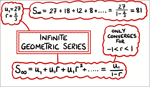
\(S_\infty = \frac{a}{1-r}\) where \(|r| < 1\).
Link to 1.3 Geometric sequences and series.
Applications could include the bouncing ball, recurring decimals, fractals, Achilles and the tortoise paradox.
Students should understand when a geometric series converges and when it diverges.
Link to limits and series in AHL topic 5.
📌 Introduction
Infinite geometric series represent one of the most beautiful and counterintuitive concepts in mathematics. While it seems impossible to add infinitely many numbers and get a finite result, infinite convergent geometric series demonstrate that this is not only possible but occurs in countless real-world phenomena. From the bouncing ball that never quite stops to the recurring decimal 0.333… = 1/3, these series help us understand how infinite processes can have finite outcomes.
Building on our knowledge of finite geometric series from SL 1.3, we now explore what happens when we extend the series to infinity. The key insight is that convergence depends entirely on the common ratio r: when |r| < 1, the terms become smaller and smaller, allowing the infinite sum to approach a finite limit. This concept has profound applications in physics, finance, computer science, and pure mathematics, forming a bridge between discrete mathematics and calculus.
📌 Definition Table
Term
Definition
Infinite Geometric Series
A series of the form \(a + ar + ar^2 + ar^3 + \cdots = \sum_{n=0}^{\infty} ar^n\)
Where a is the first term and r is the common ratio
Convergence
An infinite series converges if the sum approaches a finite limit
For geometric series: converges when \(|r| < 1\)
Divergence
An infinite series diverges if the sum does not approach a finite limit
For geometric series: diverges when \(|r| \geq 1\)
Sum to Infinity
\(S_\infty = \frac{a}{1-r}\) where \(|r| < 1\)
The finite limit of an infinite convergent geometric series
Partial Sum
\(S_n = \frac{a(1-r^n)}{1-r}\) for \(r \neq 1\)
Sum of the first n terms of the series
Limit
\(\lim_{n \to \infty} S_n = S_\infty\) when the series converges
The value that the partial sums approach as n increases
Recurring Decimal
A decimal with repeating digits that can be expressed as an infinite geometric series
Example: 0.333… = 3/10 + 3/100 + 3/1000 + …
Geometric Progression
Alternative name for geometric sequence
Each term is obtained by multiplying the previous term by r
📌 Properties & Key Formulas
Convergence Test: \(\sum_{n=0}^{\infty} ar^n\) converges if and only if \(|r| < 1\)
Sum Formula: \(S_\infty = \frac{a}{1-r}\) when \(|r| < 1\)
Divergence Cases: If \(|r| \geq 1\), the series diverges to infinity
For a geometric series with first term \(a\) and common ratio \(r\) such that \(|r| < 1\):
\[
S = a + ar + ar^2 + ar^3 + \cdots = \frac{a}{1 – r}
\]
**Convergence Condition:** The series converges only when \(|r| < 1\).
🧠 Examiner Tip:Always check |r| < 1 before using the sum formula. If |r| ≥ 1, state that the series diverges.
Remember: The sum formula only applies to convergent series. For divergent series, the sum is undefined or infinite.
📌 Common Mistakes & How to Avoid Them
⚠️ Common Mistake #1: Using the sum formula when the series diverges
Wrong: For \(2 + 4 + 8 + 16 + \cdots\), using \(S_\infty = \frac{2}{1-2} = -2\) Right: Since \(|r| = 2 > 1\), the series diverges. No finite sum exists.
How to avoid: Always check the convergence condition \(|r| < 1\) first.
⚠️ Common Mistake #2: Confusing the first term when series doesn’t start with ‘a’
Wrong: For \(3 + 6 + 12 + 24 + \cdots\), using \(a = 3\) when \(r = 2\) Right: This series diverges since \(|r| = 2 > 1\)
How to avoid: Identify the correct first term and common ratio before applying any formula.
⚠️ Common Mistake #3: Incorrect handling of recurring decimals
How to avoid: Carefully identify the repeating pattern and corresponding geometric series.
⚠️ Common Mistake #4: Sign errors with alternating series
Wrong: For \(1 – \frac{1}{2} + \frac{1}{4} – \frac{1}{8} + \cdots\), using \(r = \frac{1}{2}\) Right: The common ratio is \(r = -\frac{1}{2}\), so \(S_\infty = \frac{1}{1-(-\frac{1}{2})} = \frac{2}{3}\)
How to avoid: Pay careful attention to alternating signs – they indicate a negative common ratio.
⚠️ Common Mistake #5: Confusing infinite series with finite series formulas
Wrong: Using \(S_n = \frac{a(1-r^n)}{1-r}\) for infinite series Right: For infinite convergent series, use \(S_\infty = \frac{a}{1-r}\) where \(|r| < 1\)
How to avoid: Remember that infinite series require taking the limit as n → ∞.
📌 Calculator Skills: Casio CG-50 & TI-84
📱 Using Casio CG-50 for Infinite Series
Testing Convergence:
1. Calculate several partial sums to observe the pattern
2. Use TABLE function to generate terms: Y1 = A*R^X
3. Use SEQ function: seq(2*(0.5)^X, X, 0, 20) for first 21 terms
4. Use SUM function to add partial sums
Recurring Decimals:
1. Enter the decimal: 0.333333333…
2. Use [OPTN] → [NUM] → [►Frac] to convert to fraction
3. Verify: 1÷3 = 0.333…
Graphical Verification:
1. Graph Y1 = sum of first X terms
2. Use [TRACE] to see how sum approaches limit
3. Graph Y2 = theoretical sum for comparison
Series Computation:
1. Use [MENU] → “Sequence” for generating terms
2. Store partial sums: SUM(SEQ(…))
3. Compare with formula: A/(1-R)
📱 Using TI-84 for Infinite Series
Sequence and Series Operations:
1. [2nd] [STAT] → “OPS” → [5:seq(] for sequences
2. seq(2*.5^X, X, 0, 20) generates terms
3. [2nd] [STAT] → “MATH” → [5:sum(] to add them
4. sum(seq(2*.5^X, X, 0, N)) for partial sums
Fraction Conversion:
1. Enter decimal: 0.181818…
2. [MATH] → [1:►Frac] converts to fraction
3. Check: 2/11 = 0.181818…
Graphical Analysis:
1. [Y=] → Y1 = sum(seq(…, X, 0, X))
2. Use [WINDOW] to set appropriate range
3. [TRACE] to see convergence behavior
Programming for Series:
1. [PRGM] → [NEW] to create program
2. Use loops to compute partial sums
3. Display convergence to theoretical value
📱 Verification and Analysis Tips
Convergence testing:
• Compute S₁₀, S₂₀, S₅₀ to see if approaching limit
• Compare with theoretical S∞ = a/(1-r)
• Check that |r| < 1 for convergence
Error analysis:
• Calculate |S_n – S_∞| for different n values
• Observe exponential decrease in error
• Use this for approximation accuracy
Real-world modeling:
• Store parameters in variables
• Use series for compound interest problems
• Model bouncing ball heights
📌 Mind Map
📌 Applications in Science and IB Math
Physics: Damped oscillations, radioactive decay series, light intensity through filters
Economics: Perpetual annuities, economic multiplier effects, present value calculations
Computer Science: Algorithm analysis, data compression, fractals and computer graphics
Engineering: Signal processing, control systems, electrical circuits with capacitors
Biology: Population dynamics, pharmacokinetics, ecosystem energy transfer
Number Theory: Recurring decimals, p-adic numbers, continued fractions
Pure Mathematics: Real analysis, topology, function series, Fourier analysis
➗ IA Tips & Guidance:Infinite geometric series offer fascinating opportunities for exploring the connection between finite and infinite mathematics.
Excellent IA Topics:
• Mathematical analysis of the bouncing ball problem with air resistance
• Fractal geometry and self-similarity using infinite geometric series
• Economic modeling: perpetual annuities and their real-world applications
• Zeno’s paradoxes: mathematical resolution using infinite series
• Recurring decimals: establishing the connection between fractions and infinite series
• Koch snowflake: perimeter and area calculations using infinite series
• Musical mathematics: harmonic series and frequency relationships
• Population genetics: allele frequency changes over infinite generations
IA Structure Tips:
• Start with concrete examples before moving to abstract theory
• Use calculator/computer verification of theoretical results
• Include historical context (Zeno, Achilles and the tortoise)
• Connect to real-world phenomena and practical applications
• Explore the philosophical implications of infinite processes
• Compare different types of series (geometric vs arithmetic)
• Use graphical representations to illustrate convergence
• Discuss the mathematical rigor behind infinite limits
📌 Worked Examples (IB Style)
Q1. Find the sum to infinity of the series: \(\frac{1}{3} + \frac{1}{9} + \frac{1}{27} + \frac{1}{81} + \cdots\)
Solution:
Step 1: Identify the first term and common ratio
First term: \(a = \frac{1}{3}\)
To find r: \(r = \frac{\text{second term}}{\text{first term}} = \frac{1/9}{1/3} = \frac{1}{9} \times \frac{3}{1} = \frac{1}{3}\)
Step 2: Check for convergence
\(|r| = \left|\frac{1}{3}\right| = \frac{1}{3} < 1\)
Since |r| < 1, the series converges.
Step 3: Apply the sum formula
\(S_\infty = \frac{a}{1-r} = \frac{1/3}{1-1/3} = \frac{1/3}{2/3} = \frac{1}{3} \times \frac{3}{2} = \frac{1}{2}\)
✅ Sum to infinity = \(\frac{1}{2}\)
Q2. Express the recurring decimal \(0.272727…\) as a fraction.
Solution:
Step 1: Express as an infinite geometric series
\(0.272727… = 0.27 + 0.0027 + 0.000027 + \cdots\)
\(= \frac{27}{100} + \frac{27}{10000} + \frac{27}{1000000} + \cdots\)
Step 2: Identify first term and common ratio
First term: \(a = \frac{27}{100}\)
Common ratio: \(r = \frac{27/10000}{27/100} = \frac{27}{10000} \times \frac{100}{27} = \frac{1}{100}\)
Step 3: Check convergence and find sum
\(|r| = \frac{1}{100} < 1\), so the series converges.
\(S_\infty = \frac{27/100}{1-1/100} = \frac{27/100}{99/100} = \frac{27}{100} \times \frac{100}{99} = \frac{27}{99} = \frac{3}{11}\)
✅ \(0.272727… = \frac{3}{11}\)
Q3. A ball is dropped from a height of 10m. After each bounce, it reaches 60% of its previous height. Find the total distance traveled by the ball.
Solution:
Step 1: Analyze the motion
• Initial drop: 10m downward
• First bounce: 6m up, then 6m down
• Second bounce: 3.6m up, then 3.6m down
• Third bounce: 2.16m up, then 2.16m down
• And so on…
Step 2: Set up the series
Total distance = Initial drop + Sum of all up distances + Sum of all down distances
Total distance = 10 + (6 + 3.6 + 2.16 + …) + (6 + 3.6 + 2.16 + …)
Total distance = 10 + 2(6 + 3.6 + 2.16 + …)
Step 3: Find the sum of bounce heights
For the series 6 + 3.6 + 2.16 + …
First term: a = 6, Common ratio: r = 0.6
Since |r| = 0.6 < 1, the series converges.
Sum = \(\frac{6}{1-0.6} = \frac{6}{0.4} = 15\)
Step 4: Calculate total distance
Total distance = 10 + 2(15) = 10 + 30 = 40m
✅ Total distance = 40m
Q4. Find the sum to infinity of: \(8 – 4 + 2 – 1 + \frac{1}{2} – \frac{1}{4} + \cdots\)
Solution:
Step 1: Identify the pattern
This is an alternating geometric series.
First term: \(a = 8\)
To find r: \(r = \frac{-4}{8} = -\frac{1}{2}\)
Step 3: Check convergence
\(|r| = \left|-\frac{1}{2}\right| = \frac{1}{2} < 1\)
The series converges.
Step 4: Apply sum formula
\(S_\infty = \frac{a}{1-r} = \frac{8}{1-(-\frac{1}{2})} = \frac{8}{1+\frac{1}{2}} = \frac{8}{\frac{3}{2}} = 8 \times \frac{2}{3} = \frac{16}{3}\)
✅ Sum to infinity = \(\frac{16}{3}\)
Q5. A perpetual annuity pays $1000 at the end of each year. If the interest rate is 5% per year, find the present value.
Solution:
Step 1: Set up present value calculation
Present value of payments:
• Year 1: \(\frac{1000}{1.05}\)
• Year 2: \(\frac{1000}{(1.05)^2}\)
• Year 3: \(\frac{1000}{(1.05)^3}\)
• And so on…
Step 3: Identify series parameters
First term: \(a = \frac{1}{1.05}\)
Common ratio: \(r = \frac{1}{1.05} = \frac{1}{1.05} \approx 0.952\)
Since |r| < 1, the series converges.
Step 4: Calculate present value
Sum of series = \(\frac{1/1.05}{1-1/1.05} = \frac{1/1.05}{(1.05-1)/1.05} = \frac{1/1.05}{0.05/1.05} = \frac{1}{0.05} = 20\)
Therefore: PV = \(1000 \times 20 = \$20,000\)
✅ Present value = $20,000
📝 Paper Tip:Always state clearly whether a series converges or diverges before attempting to find its sum.
Key problem-solving steps:
• Identify the first term and common ratio
• Check convergence condition |r| < 1
• Apply sum formula only if convergent
• For divergent series, state that no finite sum exists
• For word problems, set up the series carefully
• Verify your answer makes sense in context
📌 Extended Response Questions (with Full Solutions)
Q1. A savings scheme works as follows: $100 is invested at the start, then $90 at the end of the first year, $81 at the end of the second year, and so on, with each payment being 90% of the previous year’s payment.
(a) Show that this forms a geometric series. [2 marks]
(b) If this continues indefinitely, find the total amount invested. [3 marks]
(c) If the investment earns 6% annual interest, find the present value of all future payments. [4 marks]
This question bank contains 17 questions covering advanced laws of exponents and rational logarithmic operations, distributed across different paper types according to IB AAHL curriculum standards.
Equality occurs when \(2^x = 2^{-x}\), i.e., when \(x = 0\)
Check: \(f(0) = 2^0 + 2^0 = 1 + 1 = 2\)
✅ Final Answers:
(a) Proven: f(x) is even
(b) f(1) = 2.5, f(2) = 4.25
(c) \(x = \log_2\left(\frac{5 \pm \sqrt{21}}{2}\right)\)
(d) Minimum value is 2 at x = 0
Paper 3 – Q5. The magnitude of sound intensity is measured using \(L = 10\log\left(\frac{I}{I_0}\right)\) decibels, where \(I_0 = 10^{-12}\) W/m² is the reference intensity.
(a) A whisper has intensity \(I = 10^{-10}\) W/m². Find its sound level in decibels. [2 marks]
(b) A rock concert measures 110 dB. Find the intensity of sound. [3 marks]
(c) How many times more intense is the rock concert compared to the whisper? [2 marks]
(d) If two identical sound sources are combined, show that the total sound level increases by approximately 3 dB. [4 marks]
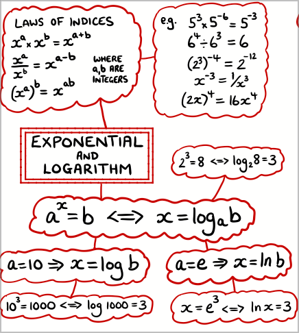
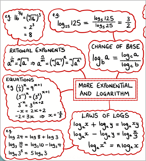
Solving exponential equations, including ones where logs are needed.
Solving logarithmic equations.
Using logarithms to solve exponential equations, and exponentials to solve logarithmic equations.
Graph of \(y = a^x\), \(a > 0\), \(a ≠ 1\) and its inverse \(y = \log_a x\).
Extension of laws of exponents to rational exponents \(x^{p/q}\).
Students should be able to solve exponential and logarithmic equations analytically where possible.
Use of technology to solve more complex exponential and logarithmic equations.
The relationship \(x^{p/q} = \sqrt[q]{x^p} = (\sqrt[q]{x})^p\) should be understood.
Link to exponential and logarithmic functions in topic 2.
📌 Introduction
Building on the foundations of SL 1.5, this topic extends the laws of exponents to include rational exponents and develops more sophisticated techniques for solving exponential and logarithmic equations. Rational exponents provide a unified way to express both powers and roots, while advanced logarithmic techniques enable us to solve complex exponential equations that arise in real-world applications.
The inverse relationship between exponential and logarithmic functions becomes crucial for solving equations where the unknown appears as an exponent. This topic also introduces the graphical representation of exponential and logarithmic functions, highlighting their inverse relationship through reflection across the line \(y = x\). These concepts form the mathematical foundation for modeling exponential growth and decay phenomena across multiple scientific disciplines.
📌 Definition Table
Term
Definition
Rational Exponent
An exponent that can be expressed as a fraction \(\frac{p}{q}\) where p and q are integers, \(q ≠ 0\)
\(x^{p/q} = \sqrt[q]{x^p} = (\sqrt[q]{x})^p\)
Principal Root
For \(x^{1/n} = \sqrt[n]{x}\), the principal nth root is the positive root when x > 0
Example: \(16^{1/4} = 2\) (not -2)
Exponential Equation
An equation where the unknown appears as an exponent
Examples: \(3^x = 27\), \(2^{x+1} = 5^{x-2}\)
Logarithmic Equation
An equation involving logarithms of the unknown
Examples: \(\log_2(x + 3) = 5\), \(\log x + \log(x – 1) = 1\)
Inverse Functions
\(f(x) = a^x\) and \(g(x) = \log_a x\) are inverse functions
Their graphs are reflections of each other across \(y = x\)
Domain and Range
For \(y = a^x\): Domain = ℝ, Range = (0, ∞)
For \(y = \log_a x\): Domain = (0, ∞), Range = ℝ
Asymptote
\(y = a^x\) has horizontal asymptote \(y = 0\)
\(y = \log_a x\) has vertical asymptote \(x = 0\)
Exponential Growth/Decay
If a > 1: exponential growth
If 0 < a < 1: exponential decay
How to avoid: Factor expressions before applying log laws; \(\log(a + b) ≠ \log a + \log b\).
⚠️ Common Mistake #4: Losing solutions when solving exponential equations
Wrong: From \(4^x = 2^{x+3}\), concluding \((2^2)^x = 2^{x+3}\), so \(2x = x + 3\), thus \(x = 3\) Right: This is actually correct! But check: \(4^3 = 64\) and \(2^{3+3} = 2^6 = 64\) ✓
How to avoid: Always substitute your solution back into the original equation to verify.
⚠️ Common Mistake #5: Confusion with negative bases and fractional exponents
Wrong: \((-8)^{2/3} = [(-8)^2]^{1/3} = 64^{1/3} = 4\) Right: \((-8)^{2/3}\) is undefined in real numbers for most purposes
How to avoid: Restrict domains to positive numbers for fractional exponents unless specifically dealing with complex numbers.
📌 Calculator Skills: Casio CG-50 & TI-84
📱 Using Casio CG-50 for Advanced Exponents & Logarithms
Rational Exponents:
1. Use parentheses: 8^(2/3) gives correct result
2. Use fractional form: 8^(2÷3) also works
3. Alternative: 8^(0.6666…) gives decimal approximation
4. For roots: 8^(1/3) or use [SHIFT] [x√] for cube roots
Solving Exponential Equations:
1. Use [MENU] → “Equation/Func” → “Solve”
2. Enter equation like: 2^X – 5^(X-1) = 0
3. Or use [MENU] → “Graph & Table” to find intersections
Advanced Logarithms:
1. Natural log: [ln] key
2. Common log: [log] key
3. General base: log₂(8) = ln(8)/ln(2)
4. Check solutions by substitution
Graphing Functions:
1. Graph Y₁ = 2^X and Y₂ = log₂(X) to see inverse relationship
2. Use [SHIFT] [MENU] to access transformation options
📱 Using TI-84 for Advanced Exponents & Logarithms
Rational Exponents:
1. Use [^] with parentheses: 8^(2/3)
2. Alternative notation: 8^(2÷3) using [÷] key
3. For roots: [2nd] [√] for square root, or [MATH] → [4:∛(] for cube root
Solving Equations:
1. [MATH] → [0:Solver] for single equations
2. Enter: 0 = 2^X – 16
3. Or use intersect method with graphs
Logarithm Functions:
1. [LOG] for base 10
2. [LN] for natural logarithm
3. Change of base: LOG(8)/LOG(2) for log₂(8)
4. Store intermediate results: [STO→] [ALPHA] [A]
Graphical Analysis:
1. [Y=] to enter functions
2. [ZOOM] → [6:ZStandard] for good viewing window
3. [2nd] [CALC] → [5:intersect] to find solutions
4. Use [TRACE] to verify solutions
📱 Verification and Error-Checking Tips
Always verify solutions:
• Substitute back into original equations
• Check domain restrictions (no negative logs)
• Use different methods to confirm results
Common calculator pitfalls:
• Order of operations with parentheses
• Rounding errors in intermediate steps
• Incorrect window settings for graphs
Professional techniques:
• Store exact fractions when possible
• Use multiple approaches (algebraic, graphical, numerical)
• Keep more decimal places in intermediate calculations
📌 Mind Map
📌 Applications in Science and IB Math
Physics: Radioactive decay with half-life calculations, Newton’s law of cooling
Chemistry: Chemical reaction kinetics, pH calculations with buffer systems
Biology: Population growth models, enzyme kinetics, allometric relationships
Economics: Compound interest with continuous compounding, inflation models
Engineering: Signal processing, exponential filtering, control system analysis
Geology: Carbon dating, earthquake magnitude scales, geological time
Medicine: Drug concentration decay, dosage calculations, epidemiological models
Computer Science: Algorithm complexity analysis, information theory, data compression
➗ IA Tips & Guidance:Advanced exponential and logarithmic functions offer rich opportunities for investigating real-world phenomena.
Excellent IA Topics:
• Carbon dating accuracy and mathematical modeling
• Comparing different population growth models (exponential vs logistic)
• Mathematical analysis of music and logarithmic frequency scales
• Investment strategies: comparing different compounding methods
• Drug dosage optimization using exponential decay models
• Earthquake prediction using logarithmic magnitude relationships
• Sound intensity and decibel scale mathematical analysis
• Cooling/heating curves and Newton’s law applications
IA Structure Tips:
• Collect real data and fit exponential/logarithmic models
• Use advanced calculator features for complex curve fitting
• Compare different bases and their effects on modeling accuracy
• Investigate limiting behaviors and asymptotic properties
• Include sensitivity analysis for parameter variations
• Connect mathematical results to practical implications
• Use graphical analysis to support analytical findings
📝 Paper Tip:Always check domain restrictions when solving logarithmic equations, and verify solutions by substitution.
Key solving strategies:
• Express exponential equations with common bases when possible
• Use substitution for exponential equations that become quadratic
• Apply logarithm laws carefully and check domains
• Convert between exponential and logarithmic forms as needed
• Use technology to verify complex solutions
• Be aware of extraneous solutions introduced during solving