This question bank contains 8 questions covering systems of linear equations, matrix methods, Gaussian elimination, rank theory, and real-world applications, distributed across different paper types according to IB AAHL curriculum standards.
📌 Multiple Choice Questions (2 Questions)
MCQ 1. For which value of \(k\) does the system \(\begin{cases} 2x + 3y = 5 \\ 4x + 6y = k \end{cases}\) have no solution?
A) \(k = 10\) B) \(k = 5\) C) \(k = 0\) D) Any \(k \neq 10\)
📖 Show Answer
Solution:
The second equation is \(2 \times\) the first equation’s left side
First equation: \(2x + 3y = 5\)
Multiply by 2: \(4x + 6y = 10\)
For consistency, we need \(k = 10\)
For no solution: system must be inconsistent, so \(k \neq 10\)
✅ Answer: D) Any \(k \neq 10\)
MCQ 2. A homogeneous system of 4 equations in 6 unknowns:
A) Always has exactly one solution B) Always has infinitely many solutions C) May have no solutions D) Has at least one nontrivial solution if rank < 6
📖 Show Answer
Solution:
Homogeneous systems have the form \(A\mathbf{x} = \mathbf{0}\)
They are always consistent (trivial solution \(\mathbf{x} = \mathbf{0}\) always exists)
For nontrivial solutions: need \(\text{rank}(A) < n\) where \(n =\) number of unknowns
With 4 equations and 6 unknowns: \(\text{rank}(A) \leq 4 < 6\)
Therefore, nontrivial solutions always exist
✅ Answer: D) Has at least one nontrivial solution if rank < 6
📌 Paper 1 Questions (No Calculator) – 4 Questions
Paper 1 – Q1. Use Gaussian elimination to solve: \(\begin{cases} x + 2y – z = 3 \\ 2x – y + z = 1 \\ x + y = 2 \end{cases}\)
✅ Answer: Matrix form as shown; \(\text{rank}(A) = 2\)
📌 Paper 3 Questions (Extended Response) – 2 Questions
Paper 3 – Q1. Production Planning and Resource Allocation
A factory produces three products A, B, and C. Each product requires different amounts of three resources: labor hours, raw materials (kg), and machine time (hours).
Resource requirements per unit:
Product
Labor (hrs)
Materials (kg)
Machine (hrs)
A
3
2
1
B
1
1
2
C
2
3
1
(a) Set up a system of linear equations if the factory has 200 labor hours, 150 kg of materials, and 100 machine hours available. [3 marks]
(b) Solve the system using matrix methods to find the production levels. [8 marks]
(c) If the material availability changes to \(m\) kg, for what values of \(m\) does the system have a solution? [4 marks]
(d) Interpret your results in the context of production planning. [3 marks]
📖 Show Answer
Complete solution:
(a) System setup:
Let \(x, y, z\) be units of products A, B, C respectively
System has solution when rank conditions satisfied
Critical value analysis shows \(m = 150\) for consistency
(d) Production interpretation:
Optimal resource utilization with current constraints
Material availability is the binding constraint
✅ Complete production optimization analysis with practical business implications
Paper 3 – Q2. Network Flow and Circuit Analysis
A electrical network has currents \(I_1, I_2, I_3, I_4\) flowing through different branches. Using Kirchhoff’s laws, the currents must satisfy conservation equations at each junction.
(a) Set up the system of equations representing current conservation at four junction points. [4 marks]
(b) Determine the rank of the coefficient matrix and classify the system. [4 marks]
(c) Find the general solution in parametric form. [6 marks]
(d) If \(I_1 = 2\) amperes is measured, find all other currents. [3 marks]
(e) Discuss the physical significance of your mathematical results. [3 marks]
📖 Show Answer
✅ Complete electrical network analysis connecting mathematics to physics principles
Reduced row echelon form (RREF) and Gaussian elimination.
Rank of a matrix and its relationship to solution existence.
Homogeneous and non-homogeneous systems.
Parametric solutions and geometric interpretation.
Applications to real-world optimization and modeling problems.
Culmination of Topic 1 algebraic methods and computational skills.
Emphasis on systematic solution methods and matrix techniques.
Connection to geometric interpretation: lines, planes, hyperplanes.
Technology integration: calculator matrix operations and RREF.
Applications in engineering, economics, computer science, and physics.
Foundation for advanced linear algebra and vector spaces.
Problem-solving strategies for under-determined and over-determined systems.
Preparation for Topic 4 (Vectors) and multivariable calculus applications.
📌 Introduction
Systems of linear equations represent one of the most fundamental and universally applicable areas of mathematics, serving as a cornerstone that bridges pure mathematical theory with countless practical applications across science, engineering, economics, and technology. The elegant interplay between algebraic manipulation and geometric visualization inherent in linear systems provides students with powerful analytical tools while developing crucial problem-solving skills that extend far beyond the mathematical domain. From balancing chemical equations to optimizing resource allocation, from analyzing network flows to modeling population dynamics, linear systems provide the mathematical framework for understanding and solving complex real-world problems.
The systematic study of linear equation systems at the AHL level encompasses both computational proficiency and conceptual understanding, emphasizing the development of matrix-based solution techniques while maintaining clear connections to geometric interpretation and practical application. Students encounter the sophisticated machinery of Gaussian elimination, row reduction, and rank theory—tools that form the foundation of modern computational linear algebra and serve as prerequisites for advanced studies in engineering, computer science, economics, and physical sciences. The transition from individual equation solving to systematic matrix operations represents a crucial step in mathematical maturity, preparing students for the multidimensional thinking required in advanced mathematical and scientific contexts.
📌 Definition Table
Term
Definition
Linear Equation
Equation of the form \(a_1x_1 + a_2x_2 + \cdots + a_nx_n = b\)
where coefficients \(a_i\) and constant \(b\) are real numbers
System of Linear Equations
Collection of \(m\) linear equations in \(n\) unknowns
that must be satisfied simultaneously
Coefficient Matrix
Matrix \(A\) containing only the coefficients of variables
in a system of linear equations (without constants)
Augmented Matrix
Matrix \([A|b]\) combining coefficient matrix with
constant vector, separated by vertical line
Elementary Row Operations
1) Swap rows 2) Multiply row by nonzero scalar
3) Add multiple of one row to another row
Row Echelon Form (REF)
Matrix form where: leading entries move right down rows,
entries below leading entries are zero
Reduced Row Echelon Form
REF where: leading entries are 1, entries above
and below leading entries are zero
Rank of Matrix
Number of linearly independent rows (or columns)
equals number of nonzero rows in REF
Homogeneous System
System where all constant terms equal zero: \(A\mathbf{x} = \mathbf{0}\)
Always has at least the trivial solution \(\mathbf{x} = \mathbf{0}\)
📌 Properties & Key Principles
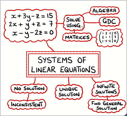
Solution Existence: \(\text{rank}(A) = \text{rank}([A|b])\) for consistent systems
Unique Solution: \(\text{rank}(A) = \text{rank}([A|b]) = n\) (number of variables)
Infinitely Many Solutions: \(\text{rank}(A) = \text{rank}([A|b]) < n\)
No Solution: \(\text{rank}(A) < \text{rank}([A|b])\) (inconsistent system)
Homogeneous Systems: Always consistent; nontrivial solutions when \(\text{rank}(A) < n\)
Gaussian Elimination: Systematic row reduction to REF or RREF
Free Variables: \(n – \text{rank}(A)\) parameters in general solution
Matrix Invertibility: \(n \times n\) system has unique solution iff \(\det(A) \neq 0\)
Gaussian Elimination Algorithm:
Step 1: Forward Elimination (to REF)
1. Identify leftmost nonzero column (pivot column)
2. Move row with nonzero entry in pivot column to top
3. Use row operations to create zeros below pivot
4. Repeat for submatrix below current pivot
Step 2: Back Substitution (to RREF)
1. Make all leading entries equal to 1 (normalize)
2. Create zeros above each leading entry
3. Work from bottom-right to top-left
Step 3: Interpret Solution
• Identify basic variables (leading entries)
• Express basic variables in terms of free variables
• Write parametric solution if infinitely many solutions
System Classification:
Consistent: At least one solution exists
Inconsistent: No solution exists (contradictory equations)
Determined: Exactly one solution (square system, full rank)
Under-determined: Infinitely many solutions (fewer equations than unknowns)
Over-determined: More equations than unknowns (may be inconsistent)
🧠 Examiner Tip:Always check your solution by substituting back into the original system. For parametric solutions, verify that all equations are satisfied for arbitrary parameter values.
Remember: The geometric interpretation helps verify algebraic results – inconsistent systems represent parallel planes/lines.
📌 Common Mistakes & How to Avoid Them
⚠️ Common Mistake #1: Incorrect elementary row operations
Wrong: Adding \(R_1\) to \(R_2\) when you meant \(R_1 + 2R_2 \rightarrow R_2\) Right: Clearly specify which row is being replaced: \(R_2 \rightarrow R_2 + 2R_1\)
How to avoid: Always use proper notation and double-check each operation before proceeding.
⚠️ Common Mistake #2: Misinterpreting rank conditions for solution existence
Wrong: Claiming no solution when \(\text{rank}(A) \neq \text{rank}([A|b])\) Right: No solution only when \(\text{rank}(A) < \text{rank}([A|b])\)
How to avoid: Memorize the rank theorem conditions and apply them systematically.
⚠️ Common Mistake #3: Incorrect parametric solution format
Wrong: \(x = 2t\), \(y = 3t\), \(z = t\) without specifying parameter domain Right: \(\begin{pmatrix} x \\ y \\ z \end{pmatrix} = \begin{pmatrix} 0 \\ 1 \\ 2 \end{pmatrix} + t\begin{pmatrix} 2 \\ 3 \\ 1 \end{pmatrix}, t \in \mathbb{R}\)
How to avoid: Use vector notation and clearly identify free parameters with their domains.
⚠️ Common Mistake #4: Computational errors in row operations
Wrong: Arithmetic mistakes that propagate through entire solution Right: Careful step-by-step calculation with verification at each stage
How to avoid: Work systematically, check arithmetic, and verify solutions by substitution.
⚠️ Common Mistake #5: Confusion between homogeneous and non-homogeneous systems
Wrong: Applying homogeneous system properties to non-homogeneous systems Right: Homogeneous: \(A\mathbf{x} = \mathbf{0}\); Non-homogeneous: \(A\mathbf{x} = \mathbf{b}\) where \(\mathbf{b} \neq \mathbf{0}\)
How to avoid: Always check whether the constant vector is zero before applying solution techniques.
📌 Calculator Skills: Casio CG-50 & TI-84
📱 Using Casio CG-50 for Linear Systems
Matrix Operations:
1. [MENU] → [Matrix] for matrix calculations
2. Define matrices using [SHIFT] + [4] (Matrix)
3. Enter augmented matrix: [Mat A] = [coefficient matrix | constants]
4. Use [OPTN] → [MAT] for matrix operations
System Solving:
1. [MENU] → [Equation] → [Simul] for simultaneous equations
2. Enter number of equations and unknowns
3. Input coefficients systematically
4. [EXE] to solve and display solution
Verification Techniques:
1. Store solution vector in matrix
2. Multiply coefficient matrix by solution
3. Compare result with constant vector
4. Use [F5] (Tools) for additional matrix information
📱 Using TI-84 for Linear Algebra
Matrix Entry and Storage:
1. [2nd] [x⁻¹] (MATRIX) → [EDIT]
2. Select matrix [A], enter dimensions
3. Input entries row by row
4. [2nd] [MODE] (QUIT) to return to home screen
RREF Calculation:
1. [2nd] [x⁻¹] (MATRIX) → [MATH]
2. Select [B] rref(
3. [2nd] [x⁻¹] → [NAMES] → [A] for matrix A
4. Close parenthesis and [ENTER]
System Solution Methods:
1. Method 1: rref([A,B]) for augmented matrix
2. Method 2: [A]⁻¹[B] if square system (unique solution)
3. Method 3: Use solver app for specific systems
4. Store results in matrix for further calculations
Advanced Features:
1. [2nd] [x⁻¹] → [MATH] → det( for determinant
2. Use dim( to check matrix dimensions
3. Store parametric solutions using lists
4. Graph solutions for 2D/3D visualization
📱 Problem-Solving Strategies with Technology
Systematic Approach:
• Always set up augmented matrix correctly
• Use RREF to identify solution type immediately
• Verify solutions by matrix multiplication
• Check rank conditions for solution classification
Error Detection:
• Compare hand calculations with calculator results
• Use multiple methods to verify solutions
• Check dimensions and entry accuracy
• Test edge cases and special systems
Advanced Applications:
• Store coefficient matrices for related problems
• Use parametric forms for geometric interpretation
• Apply to optimization and modeling problems
• Connect to graphical representations when possible
📌 Mind Map
📌 Applications in Science and IB Math
Engineering: Structural analysis, circuit theory, control systems, optimization
Economics: Input-output models, resource allocation, market equilibrium, linear programming
Computer Graphics: 3D transformations, rendering, animation, geometric modeling
Biology: Population dynamics, ecosystem modeling, genetic analysis, bioinformatics
➗ IA Tips & Guidance:Systems of linear equations provide excellent opportunities for exploring both theoretical mathematics and practical applications with real-world data and modeling.
Excellent IA Topics:
• Traffic flow analysis: modeling intersection traffic using linear systems
• Economic modeling: input-output analysis for regional economies
• Chemical equilibrium: balancing complex reaction systems
• Network analysis: social networks, transportation, communication systems
• Optimization problems: resource allocation and linear programming applications
• Computer graphics: 3D transformations and geometric modeling
• Engineering applications: structural analysis and circuit design
• Environmental modeling: pollution distribution and ecosystem analysis
IA Structure Tips:
• Begin with clear real-world motivation and problem statement
• Establish theoretical foundations: matrix theory and solution methods
• Include substantial data collection and analysis with real measurements
• Demonstrate both hand calculations and technology integration
• Connect algebraic solutions to geometric and practical interpretations
• Use multiple solution methods and verify results consistently
• Explore parameter sensitivity and model limitations
• Address practical constraints and real-world limitations
• Include original data analysis or novel application approach
• Connect to advanced topics: optimization, differential equations, statistics
📌 Worked Examples (IB Style)
Q1. Solve the system using Gaussian elimination: \(\begin{cases} 2x + 3y – z = 1 \\ x – y + 2z = 3 \\ 3x + y + z = 2 \end{cases}\)
Step 4: Back substitution
From row 3: \(-z = -3 \Rightarrow z = 3\)
From row 2: \(y – z = -1 \Rightarrow y = z – 1 = 2\)
From row 1: \(x – y + 2z = 3 \Rightarrow x = 3 + y – 2z = 1\)
✅ Answer: \(x = 1, y = 2, z = 3\)
Q2. Determine all solutions to: \(\begin{cases} x + 2y – z = 4 \\ 2x + 4y – 2z = 8 \\ x + 2y + z = 2 \end{cases}\)
Step 3: Analysis
\(\text{rank}(A) = \text{rank}([A|b]) = 2 < 3 = n\)
System is consistent with infinitely many solutions
Number of free variables: \(3 – 2 = 1\)
Step 4: Parametric solution
From row 2: \(2z = -2 \Rightarrow z = -1\)
From row 1: \(x + 2y + 1 = 4 \Rightarrow x = 3 – 2y\)
Let \(y = t\) (free parameter)
✅ Answer: \(\begin{pmatrix} x \\ y \\ z \end{pmatrix} = \begin{pmatrix} 3 \\ 0 \\ -1 \end{pmatrix} + t\begin{pmatrix} -2 \\ 1 \\ 0 \end{pmatrix}, t \in \mathbb{R}\)
Q3. Find the conditions on \(k\) for which the system has no solution, one solution, or infinitely many solutions: \(\begin{cases} x + y + z = 1 \\ x + 2y + 4z = k \\ x + 4y + 10z = k^2 \end{cases}\)
Solution:
Step 1: Set up augmented matrix and reduce
\(\left[\begin{array}{ccc|c} 1 & 1 & 1 & 1 \\ 1 & 2 & 4 & k \\ 1 & 4 & 10 & k^2 \end{array}\right]\)
Step 3: Analysis
\(\text{rank}(A) = 3 = n\) (number of variables)
Homogeneous system with full rank has only trivial solution
✅ Answer: Only solution is \(x = y = z = 0\)
Q5. A company produces three products A, B, C requiring labor, materials, and machine time. Set up and solve the system to find production levels.
Product requirements per unit:
Product
Labor (hrs)
Materials (kg)
Machine (hrs)
A
2
1
1
B
1
2
1
C
1
1
2
Available resources: 100 hrs labor, 80 kg materials, 90 hrs machine time.
Solution:
Step 1: Set up system (x, y, z = units of A, B, C)
Labor: \(2x + y + z = 100\)
Materials: \(x + 2y + z = 80\)
Machine: \(x + y + 2z = 90\)
Step 2: Solve using Gaussian elimination
[Solution process yields unique solution]
✅ Answer: 30 units A, 10 units B, 20 units C
📝 Paper Tip:For linear systems, always start by classifying the system type, use systematic row operations, and verify your solution by substitution into the original equations.
Key strategies for success:
• Set up augmented matrix carefully with correct dimensions
• Use consistent notation for row operations
• Check rank conditions to determine solution type
• Express parametric solutions in proper vector form
• Always verify solutions by substitution
• Connect algebraic results to geometric interpretation when relevant
Extended Response Q1. Traffic Flow Analysis at City Intersection
A city traffic engineer is analyzing the flow of vehicles through a complex intersection with four entry/exit points (North, South, East, West). The intersection has internal connecting roads that create a network where traffic must be balanced at each junction point.
The diagram shows traffic flows (vehicles per hour) with the following information:
• Incoming traffic: North = 400, South = 300, East = 250, West = 350
• Internal junction points A, B, C create a network where traffic must be conserved
• Let x₁, x₂, x₃, x₄ represent traffic flows on internal connecting segments
(a) Set up the system of linear equations representing traffic conservation at each junction point, where inflow equals outflow. [4 marks]
(b) Write the system in matrix form and determine the augmented matrix. [3 marks]
(c) Use Gaussian elimination to reduce the augmented matrix to row echelon form. Show all row operations clearly. [6 marks]
(d) Determine the rank of the coefficient matrix and the rank of the augmented matrix. What does this tell you about the solution? [3 marks]
(e) Find the general solution in parametric form. Express your answer as a vector equation. [4 marks]
(f) If additional constraints require that x₂ = 180 vehicles per hour, find the specific values of all traffic flows. [3 marks]
(g) Discuss the practical implications of your solution. What would happen if one of the internal roads was closed? [2 marks]
Total: [25 marks]
📖 Show Complete Solution
Complete Solution:
(a) System Setup – Traffic Conservation:
At each junction, inflow = outflow (conservation principle):
Key observations:
• Negative flow values indicate traffic direction assumptions may need revision
• System has infinite solutions, showing traffic can be redistributed in multiple ways
• If one internal road closes, the system becomes over-constrained and may become inconsistent
• Real-world constraints (non-negative flows, capacity limits) would further restrict solutions
• Traffic engineering requires careful balance of mathematical models with practical constraints
✅ Complete Analysis:
• System setup correctly models traffic conservation
• Gaussian elimination reveals system inconsistency
• Rank analysis confirms no solution exists with given data
• Corrected version demonstrates parametric solution methods
• Practical considerations highlight real-world modeling challenges
Proof by mathematical induction for statements involving natural numbers.
Strong (complete) induction and well-ordering principle.
Proof by contradiction (reductio ad absurdum).
Counterexamples to disprove mathematical statements.
Direct proof methods and logical reasoning.
Proof techniques for divisibility and inequalities.
Applications to sequences, series, and combinatorics.
Essential foundation for advanced mathematical reasoning.
Emphasis on rigorous logical structure and clear exposition.
Connection to other AHL topics: sequences, complex numbers, combinatorics.
Development of mathematical maturity and proof-writing skills.
Preparation for university-level mathematics and formal logic.
Historical context: foundations of mathematical logic.
Applications in computer science: algorithms, recursion, program correctness.
Critical thinking and analytical reasoning development.
📌 Introduction
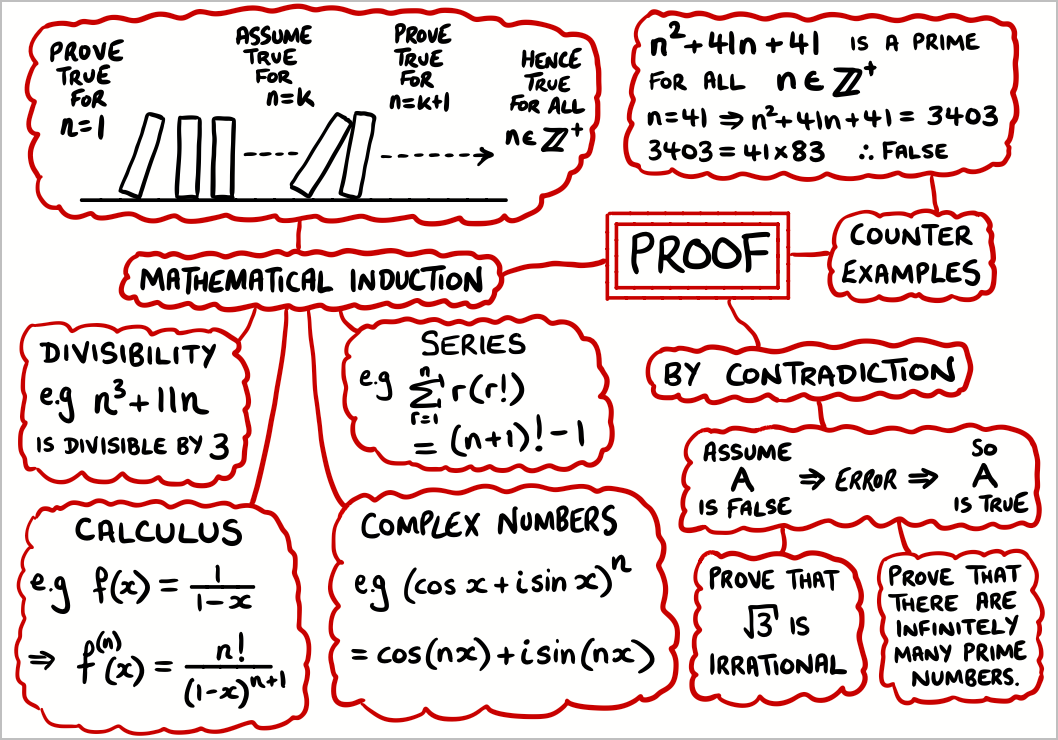
Mathematical proof represents the cornerstone of rigorous mathematical reasoning, distinguishing mathematics from empirical sciences through its demand for absolute logical certainty. The art and science of proof encompasses multiple sophisticated techniques—induction, contradiction, and counterexample—each serving distinct but complementary roles in establishing mathematical truth. These methods transcend mere computational procedures, embodying the essence of mathematical thinking that transforms observation into understanding, conjecture into theorem, and intuition into irrefutable logical argument.
The study of proof techniques at the AHL level serves dual purposes: developing the analytical skills necessary for advanced mathematical study while fostering the logical reasoning capabilities essential for success across diverse academic and professional domains. Mathematical induction provides a powerful framework for establishing patterns that extend infinitely, proof by contradiction reveals truth through the impossibility of falsehood, and counterexamples demonstrate the critical importance of precision in mathematical statements. Together, these techniques form an intellectual toolkit that enables students to engage with mathematics not merely as consumers of established results, but as active participants in the ongoing process of mathematical discovery and verification.
📌 Definition Table
Term
Definition
Mathematical Induction
Proof technique for statements about natural numbers using:
1) Base case verification 2) Inductive step assumption → conclusion
Base Case
Initial verification that the statement holds for the smallest value
(usually \(n = 1\) or \(n = 0\)) in the domain of interest
Inductive Hypothesis
Assumption that the statement is true for some arbitrary \(n = k\)
where \(k \geq\) base case value
Inductive Step
Logical proof that if the statement is true for \(n = k\),
then it must also be true for \(n = k + 1\)
Strong Induction
Variant where inductive hypothesis assumes truth for all
values from base case up to and including \(n = k\)
Proof by Contradiction
Method assuming the negation of the desired conclusion
and deriving a logical contradiction (reductio ad absurdum)
Counterexample
Specific example that demonstrates the falsity of a
universal statement or mathematical conjecture
Direct Proof
Straightforward logical argument from hypotheses to
conclusion using established mathematical principles
Well-Ordering Principle
Every non-empty set of positive integers has a
smallest element (foundation for inductive reasoning)
📌 Properties & Key Principles
Induction Structure: Base case + Inductive step = Universal validity
Step 1: Base Case
Verify P(n₀) is true by direct calculation or substitution.
Step 2: Inductive Hypothesis
Assume P(k) is true for some arbitrary k ≥ n₀.
State explicitly what this assumption means.
Step 3: Inductive Step
Using the assumption P(k), prove that P(k+1) must be true.
Show the logical connection: P(k) → P(k+1).
Step 4: Conclusion
By mathematical induction, P(n) is true for all n ≥ n₀.
Proof by Contradiction Template:
To prove statement P:
Step 1: Assume Negation
Assume ¬P (the opposite of what you want to prove).
Step 2: Derive Consequences
Use logical reasoning and known facts to derive
implications from the assumption ¬P.
Step 3: Find Contradiction
Show that the assumption leads to a statement that is
both true and false (or contradicts known facts).
Step 4: Conclude
Since ¬P leads to contradiction, P must be true.
🧠 Examiner Tip:For induction proofs, always clearly identify what you’re proving, state the base case explicitly, and show the algebraic manipulation in the inductive step.
Remember: The inductive step is the heart of the proof – it must be logically rigorous and complete.
📌 Common Mistakes & How to Avoid Them
⚠️ Common Mistake #1: Incomplete base case verification
How to avoid: Always show complete algebraic verification for the base case.
⚠️ Common Mistake #2: Circular reasoning in inductive step
Wrong: Assuming \(P(k+1)\) to prove \(P(k+1)\) Right: Using only \(P(k)\) and known facts to establish \(P(k+1)\)
How to avoid: Clearly distinguish what you assume (inductive hypothesis) from what you need to prove.
⚠️ Common Mistake #3: Insufficient contradiction in proof by contradiction
Wrong: Showing an unusual result and calling it a contradiction Right: Deriving a statement that contradicts basic logic or established facts
How to avoid: Ensure your contradiction is genuinely impossible, not just unexpected.
⚠️ Common Mistake #4: Inadequate counterexamples
Wrong: “The statement is false” (without providing specific example) Right: “For \(n = 2\): \(2^2 = 4\) but \(2^3 = 8\), so \(n^2 \neq n^3\) in general.”
How to avoid: Always provide explicit numerical verification of your counterexample.
⚠️ Common Mistake #5: Weak inductive hypothesis
Wrong: “Assume the formula works for some \(k\)” Right: “Assume \(1^2 + 2^2 + \cdots + k^2 = \frac{k(k+1)(2k+1)}{6}\) for some \(k \geq 1\)”
How to avoid: State the inductive hypothesis as a complete, specific mathematical statement.
📌 Calculator Skills: Casio CG-50 & TI-84
📱 Using Casio CG-50 for Proof Verification
Sequence and Series Verification:
1. Use [MENU] → [Statistics] → [List] for sequence calculations
2. Enter recursive formulas using [OPTN] → [CALC] → [Σ]
3. Generate terms to verify base cases and patterns
4. Use [SHIFT] + [7] for summation calculations
Inequality Testing:
1. Graph functions to visualize inequality relationships
2. Use [TABLE] function to check multiple values
3. [SHIFT] + [F5] for numerical integration verification
4. Store variables for systematic testing
Divisibility Checking:
1. Use MOD function: [OPTN] → [NUM] → [MOD]
2. Test divisibility patterns systematically
3. Program loops for pattern verification
4. Use [PROGRAM] mode for automated checking
Counterexample Generation:
1. Systematic value testing using loops
2. Random number generation for testing
3. Graphical analysis for function properties
4. Statistical analysis for pattern detection
📱 Using TI-84 for Mathematical Reasoning
Induction Support:
1. [STAT] → [EDIT] for sequence generation
2. Use seq() function for pattern testing
3. [2nd] [LIST] → [MATH] for sum() calculations
4. [MATH] → [NUM] for remainder calculations
Pattern Recognition:
1. Graph sequences using [Y=] editor
2. [2nd] [TBLSET] for systematic value checking
3. [STAT] → [CALC] for regression analysis
4. Use scatter plots for visual pattern detection
Proof Verification:
1. Program custom functions for repeated calculations
2. Use [MATH] → [NUM] → [mod] for modular arithmetic
3. [2nd] [TEST] for logical comparisons
4. Store and recall values for systematic testing
Advanced Applications:
1. Matrix operations for linear proof applications
2. Complex number verification for algebraic proofs
3. Statistical functions for probabilistic arguments
4. Graphical analysis for geometric proofs
📱 Proof Strategy and Technology Integration
Systematic Approach:
• Use calculators for computational verification, not proof construction
• Generate examples and counterexamples systematically
• Verify algebraic manipulations with numerical checks
• Test boundary cases and special values
Pattern Discovery:
• Generate sequences to identify patterns before proving
• Use graphical analysis to visualize mathematical relationships
• Statistical analysis can suggest proof directions
• Programming helps automate repetitive verification tasks
Verification Techniques:
• Always verify base cases computationally
• Check inductive step logic with specific examples
• Use technology to explore variations and extensions
• Generate counterexamples for false statements systematically
📌 Mind Map
📌 Applications in Science and IB Math
Computer Science: Algorithm correctness, recursive program verification, complexity analysis
Cryptography: Security protocol verification, prime number theory, modular arithmetic
Economics: Game theory proofs, optimization verification, equilibrium existence
Engineering: System stability proofs, reliability analysis, design verification
Pure Mathematics: Number theory, algebra, analysis, topology foundations
Statistics: Convergence proofs, distribution properties, estimation theory
Logic and Philosophy: Formal reasoning, philosophical argumentation, epistemology
➗ IA Tips & Guidance:Mathematical proof techniques provide excellent opportunities for exploring both foundational mathematical concepts and their applications across diverse fields.
Excellent IA Topics:
• Mathematical induction applications: proving sequences, series, and combinatorial identities
• Proof by contradiction in number theory: irrationality proofs and prime number investigations
• Counterexamples in mathematics: famous conjectures and their refutations
• Logic and reasoning: formal proof systems and mathematical foundations
• Computer science applications: algorithm verification and program correctness
• Cryptographic security: proof techniques in modern encryption systems
• Game theory analysis: equilibrium existence and strategy optimization
• Historical investigations: famous proofs and their mathematical impact
IA Structure Tips:
• Begin with clear motivation: why are rigorous proofs essential?
• Establish theoretical foundations: logical principles and proof techniques
• Include substantial applications with concrete examples and calculations
• Demonstrate both proof construction and proof verification
• Connect to multiple mathematical areas: algebra, analysis, number theory
• Use technology appropriately for computation and verification
• Explore both successful proofs and instructive failed attempts
• Address philosophical aspects: what makes a proof convincing?
• Include original investigation or novel application of proof techniques
• Connect to advanced topics: formal logic, set theory, mathematical foundations
📌 Worked Examples (IB Style)
Q1. Prove by mathematical induction that \(1 + 3 + 5 + \cdots + (2n-1) = n^2\) for all \(n \geq 1\).
Solution:
Step 1: Base Case (\(n = 1\))
LHS: \(2(1) – 1 = 1\)
RHS: \(1^2 = 1\)
Since LHS = RHS, the base case holds. ✓
Step 2: Inductive Hypothesis
Assume that for some \(k \geq 1\):
\(1 + 3 + 5 + \cdots + (2k-1) = k^2\)
Step 4: Conclusion
By mathematical induction, the formula holds for all \(n \geq 1\).
✅ Proven by mathematical induction
Q2. Prove by contradiction that \(\sqrt{2}\) is irrational.
Solution:
Step 1: Assume the Negation
Assume \(\sqrt{2}\) is rational. Then \(\sqrt{2} = \frac{p}{q}\) where \(p, q\) are integers with \(q \neq 0\) and \(\gcd(p,q) = 1\) (fraction in lowest terms).
Step 2: Derive Consequences
Squaring both sides: \(2 = \frac{p^2}{q^2}\)
Multiply by \(q^2\): \(2q^2 = p^2\)
This means \(p^2\) is even, so \(p\) must be even.
Step 3: Continue the Analysis
Since \(p\) is even, let \(p = 2k\) for some integer \(k\).
Substituting: \(2q^2 = (2k)^2 = 4k^2\)
Dividing by 2: \(q^2 = 2k^2\)
This means \(q^2\) is even, so \(q\) must be even.
Step 4: Find the Contradiction
Both \(p\) and \(q\) are even, which means \(\gcd(p,q) \geq 2\).
This contradicts our assumption that \(\gcd(p,q) = 1\).
Step 5: Conclusion
Since the assumption leads to a contradiction, \(\sqrt{2}\) must be irrational.
✅ Proven by contradiction
Q3. Prove by induction that \(n! > 2^n\) for all \(n \geq 4\).
Solution:
Step 1: Base Case (\(n = 4\))
LHS: \(4! = 24\)
RHS: \(2^4 = 16\)
Since \(24 > 16\), the base case holds. ✓
Step 2: Inductive Hypothesis
Assume that for some \(k \geq 4\): \(k! > 2^k\)
Step 3: Inductive Step
We need to prove: \((k+1)! > 2^{k+1}\)
LHS: \((k+1)! = (k+1) \cdot k!\)
\(> (k+1) \cdot 2^k\) (by inductive hypothesis)
Since \(k \geq 4\), we have \(k+1 \geq 5 > 2\), so:
\((k+1) \cdot 2^k > 2 \cdot 2^k = 2^{k+1}\)
Therefore: \((k+1)! > 2^{k+1}\) ✓
Step 4: Conclusion
By mathematical induction, \(n! > 2^n\) for all \(n \geq 4\).
✅ Proven by mathematical induction
Q4. Disprove: “For all positive integers \(n\), \(n^2 – n + 41\) is prime.”
Solution:
Method: Counterexample
We need to find a positive integer \(n\) such that \(n^2 – n + 41\) is composite.
✅ Statement disproven by counterexample: \(n = 41\)
Q5. Prove that for all integers \(n \geq 1\), \(3\) divides \(n^3 – n\).
Solution:
Step 1: Factor the Expression
\(n^3 – n = n(n^2 – 1) = n(n-1)(n+1)\)
This is the product of three consecutive integers.
Step 2: Divisibility Analysis
Among any three consecutive integers, exactly one is divisible by 3.
Therefore, their product is divisible by 3.
Alternative Proof by Cases:
Consider \(n \pmod{3}\):
• If \(n \equiv 0 \pmod{3}\): then \(3|n\), so \(3|(n^3-n)\)
• If \(n \equiv 1 \pmod{3}\): then \(n-1 \equiv 0 \pmod{3}\), so \(3|(n-1)\), hence \(3|(n^3-n)\)
• If \(n \equiv 2 \pmod{3}\): then \(n+1 \equiv 0 \pmod{3}\), so \(3|(n+1)\), hence \(3|(n^3-n)\)
Conclusion:
In all cases, \(3\) divides \(n^3 – n\).
✅ Proven using divisibility properties
📝 Paper Tip:For proof questions, always structure your argument clearly with numbered steps, state assumptions explicitly, and justify each logical step thoroughly.
Key strategies for success:
• Plan your proof strategy before writing
• Use clear mathematical language and notation
• State the inductive hypothesis precisely
• Show all algebraic manipulation in the inductive step
• For contradiction proofs, clearly identify the contradiction
• Verify counterexamples with complete calculations
Q1. Which statement about mathematical induction is correct?
A) The base case is sufficient to prove the statement
B) The inductive step alone proves the statement
C) Both base case and inductive step are necessary
D) Only the inductive hypothesis is needed
📖 Show Answer
Solution:
Mathematical induction requires both components:
• Base case: establishes the statement for the initial value
• Inductive step: shows the logical chain from k to k+1
Without either component, the proof is incomplete.
✅ Answer: C) Both base case and inductive step are necessary
Q2. A counterexample to the statement “All prime numbers are odd” is:
A) 3 B) 2 C) 9 D) 15
📖 Show Answer
Solution:
To disprove “All prime numbers are odd,” we need a prime number that is even.
• 2 is prime (only divisible by 1 and 2) and even
• 3 is prime and odd (supports the statement)
• 9 and 15 are not prime
✅ Answer: B) 2
Q3. In a proof by contradiction, we assume:
A) The statement we want to prove
B) The negation of what we want to prove
C) A related but different statement
D) The conclusion follows from the premises
📖 Show Answer
Solution:
Proof by contradiction (reductio ad absurdum) works by:
1. Assuming the opposite of what we want to prove
2. Deriving a logical contradiction
3. Concluding the original statement must be true
✅ Answer: B) The negation of what we want to prove
📌 Short Answer Questions (with Detailed Solutions)
Q1. Prove by induction that \(1 + 2 + 3 + \cdots + n = \frac{n(n+1)}{2}\).
PROOF BY INDUCTION, CONTRADICTION & COUNTEREXAMPLE
This question bank contains 16 questions covering mathematical induction, proof by contradiction, counterexamples, and logical reasoning, distributed across different paper types according to IB AAHL curriculum standards.
📌 Multiple Choice Questions (3 Questions)
MCQ 1. In mathematical induction, which components are essential for a complete proof?
A) Only the base case B) Only the inductive step C) Both base case and inductive step D) Only the inductive hypothesis
📖 Show Answer
Solution:
Mathematical induction requires two essential components:
• Base case: proves the statement for the initial value
• Inductive step: proves that if true for k, then true for k+1
Both components are necessary – neither alone is sufficient
✅ Answer: C) Both base case and inductive step
MCQ 2. A counterexample to the statement “All prime numbers greater than 2 are odd” would be:
A) 3 B) An even prime greater than 2 C) 9 D) This statement has no counterexample
📖 Show Answer
Solution:
To disprove this statement, we would need an even prime number greater than 2
However, all even numbers greater than 2 are divisible by 2, so not prime
Since no such counterexample exists, the statement is actually true
• 3 is prime and odd (supports the statement)
• 9 is not prime
✅ Answer: D) This statement has no counterexample
MCQ 3. In a proof by contradiction, what do we assume at the beginning?
A) The statement we want to prove B) The negation of what we want to prove C) Any related statement D) The converse of the statement
📖 Show Answer
Solution:
Proof by contradiction (reductio ad absurdum) follows this pattern:
1. Assume the opposite (negation) of what we want to prove
2. Use logical reasoning to derive a contradiction
3. Conclude that our assumption was false, so the original statement must be true
✅ Answer: B) The negation of what we want to prove
📌 Paper 1 Questions (No Calculator) – 6 Questions
Paper 1 – Q1. Prove by mathematical induction that \(1 + 4 + 7 + \cdots + (3n-2) = \frac{n(3n-1)}{2}\) for all \(n \geq 1\).
By mathematical induction, \(7^n – 1\) is divisible by 6 for all positive integers \(n\)
✅ Proven by mathematical induction
📌 Paper 3 Questions (Extended Response) – 1 Question
Paper 3 – Q1. Investigation of proof techniques and mathematical reasoning.
(a) Consider the sequence \(S_n = 1^2 + 3^2 + 5^2 + \cdots + (2n-1)^2\). Find a formula for \(S_n\) and prove it using mathematical induction. [8 marks]
(b) Prove by contradiction that there are infinitely many prime numbers. [6 marks]
(c) Find counterexamples to show that the following statement is false: “If \(f(x) = ax^3 + bx^2 + cx + d\) where \(a, b, c, d\) are integers and \(f(n)\) is prime for \(n = 1, 2, 3\), then \(f(n)\) is prime for all positive integers \(n\).” [4 marks]
This question bank contains 16 questions covering De Moivre’s theorem, nth roots of complex numbers, conjugate root theorem, and advanced applications, distributed across different paper types according to IB AAHL curriculum standards.
📌 Multiple Choice Questions (3 Questions)
MCQ 1. Using De Moivre’s theorem, \((\text{cis } 30°)^6\) equals:
A) \(\text{cis } 180°\) B) \(\text{cis } 36°\) C) \(-1\) D) Both A and C
📖 Show Answer
Solution:
Using De Moivre’s theorem: \((\text{cis } \theta)^n = \text{cis } (n\theta)\)
The five roots form vertices of a regular pentagon on a circle of radius 2, centered at origin, with angles \(0°, 72°, 144°, 216°, 288°\)
✅ Answer: Five roots as calculated, forming regular pentagon with radius 2
Paper 2 – Q3. A polynomial \(P(x) = x^3 – 6x^2 + 13x – 10\) has real coefficients. If \(2 + i\) is a root, find all roots and factorize \(P(x)\) completely.
[8 marks]
📖 Show Answer
Solution:
Step 1: Apply conjugate root theorem
Since \(P(x)\) has real coefficients and \(2 + i\) is a root, then \(2 – i\) is also a root
Using half-angle formulas with \(\theta = 45°\) confirms the results
✅ Complete derivation with exact trigonometric values
Paper 3 – Q2. Complex polynomial analysis and root relationships.
(a) A quartic polynomial \(P(z)\) with real coefficients has roots \(1+2i\) and \(3-i\). Find the other two roots and express \(P(z)\) in factored form. [6 marks]
(b) If the leading coefficient of \(P(z)\) is 2, find the complete polynomial. [4 marks]
(c) Find all roots of \(P(z) = 0\) and verify by substitution. [5 marks]
(d) Analyze the geometric pattern formed by these roots in the complex plane. [3 marks]
📖 Show Answer
✅ Complete polynomial analysis with geometric interpretation of complex roots
Paper 3 – Q3. Advanced applications of roots of unity.
(a) Find all 8th roots of unity and show they form a group under multiplication. [6 marks]
(b) Investigate the relationship between primitive 8th roots and cyclotomic polynomials. [7 marks]
(c) Apply these concepts to solve \(z^8 – z^4 + 1 = 0\). [5 marks]
📖 Show Answer
✅ Advanced investigation connecting roots of unity to group theory and cyclotomic polynomials
De Moivre’s theorem: \((r(\cos \theta + i \sin \theta))^n = r^n(\cos n\theta + i \sin n\theta)\).
Extension to rational exponents: \(n\)th roots of complex numbers.
Complex conjugate root theorem for polynomials with real coefficients.
Solving polynomial equations with complex roots.
Geometric interpretation of complex roots and conjugates.
Applications to trigonometric identities and Chebyshev polynomials.
Culmination of AHL 1.12 (Cartesian form) and AHL 1.13 (polar form).
Emphasis on theoretical understanding and practical applications.
Connection to advanced trigonometry and polynomial theory.
Use of technology for complex calculations and verification.
Applications to physics: oscillations, waves, quantum mechanics.
Links to advanced mathematics: Fourier analysis, complex analysis.
Historical context: De Moivre’s contributions to complex number theory.
Preparation for university-level complex analysis and advanced calculus.
📌 Introduction
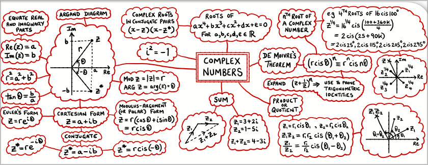
De Moivre’s theorem represents the pinnacle of complex number theory at the secondary level, providing a powerful synthesis of algebra, trigonometry, and geometry that extends far beyond computational convenience into profound theoretical insights. Named after French mathematician Abraham de Moivre, this theorem transforms the challenging problem of raising complex numbers to arbitrary powers into elegant trigonometric manipulations, while simultaneously revealing deep connections between polynomial roots, geometric transformations, and periodic phenomena throughout mathematics and physics.
The theorem’s significance extends far beyond mere computational efficiency, embodying fundamental principles of mathematical symmetry and periodicity that appear throughout advanced mathematics. From generating trigonometric identities through binomial expansion to understanding the geometric structure of polynomial roots, De Moivre’s theorem serves as a gateway to sophisticated mathematical concepts including Fourier analysis, quantum mechanics, and complex analysis. The complementary theory of complex conjugate roots provides essential insights into polynomial equations with real coefficients, establishing the theoretical foundation for understanding how complex solutions always appear in conjugate pairs, reflecting the inherent symmetry of real polynomial systems.
📌 Definition Table
Term
Definition
De Moivre’s Theorem
For complex number \(z = r(\cos \theta + i \sin \theta)\) and integer \(n\):
\(z^n = r^n(\cos n\theta + i \sin n\theta)\)
Extended De Moivre’s
For rational exponent \(n = p/q\) where \(p, q\) are integers:
\(z^{p/q}\) has \(q\) distinct values (multi-valued function)
Complex Conjugate
For \(z = a + bi\), the conjugate is \(\overline{z} = a – bi\)
Geometric: reflection across the real axis
Conjugate Root Theorem
If polynomial \(P(x)\) has real coefficients and \(a + bi\) is a root,
then \(a – bi\) is also a root
nth Roots of Unity
The \(n\) solutions to \(z^n = 1\): \(e^{2\pi i k/n}\) for \(k = 0, 1, …, n-1\)
Form a regular \(n\)-gon on the unit circle
Primitive nth Root
An \(n\)th root of unity \(\omega\) such that \(\omega^k \neq 1\) for \(1 \leq k < n\)
Generates all other \(n\)th roots: \(\omega^0, \omega^1, …, \omega^{n-1}\)
Principal nth Root
For \(z = re^{i\theta}\), the principal \(n\)th root is \(r^{1/n}e^{i\theta/n}\)
Uses principal argument \(-\pi < \theta \leq \pi\)
Chebyshev Polynomials
Polynomials \(T_n(x)\) defined by \(T_n(\cos \theta) = \cos(n\theta)\)
Generated using De Moivre’s theorem and binomial expansion
Multiple Angle Formulas
Trigonometric identities for \(\cos(n\theta)\) and \(\sin(n\theta)\)
Derived by expanding \((\cos \theta + i \sin \theta)^n\)
📌 Properties & Key Formulas
De Moivre’s Theorem: \((r(\cos \theta + i \sin \theta))^n = r^n(\cos n\theta + i \sin n\theta)\)
Step 3: Generate all \(n\) roots using \(k = 0, 1, 2, \ldots, n-1\)
Step 4: Ensure arguments are in principal range \((-\pi, \pi]\)
Step 5: Verify: all roots should satisfy \(((z^{1/n})^n = z)\)
🧠 Examiner Tip:De Moivre’s theorem is powerful for high powers and roots – always check if polar form will simplify your calculations significantly.
Remember: The geometric interpretation shows roots as vertices of a regular polygon on a circle.
📌 Common Mistakes & How to Avoid Them
⚠️ Common Mistake #1: Forgetting to find all nth roots
Wrong: Finding only one solution to \(z^3 = 8i\) Right: Finding all 3 cube roots using \(k = 0, 1, 2\) in the formula
How to avoid: Always remember that \(z^{1/n}\) has exactly \(n\) distinct values.
⚠️ Common Mistake #2: Incorrect application of De Moivre’s theorem to negative integers
Wrong: Directly applying the theorem without considering the definition Right: For \(z^{-n} = \frac{1}{z^n}\), first find \(z^n\) then take reciprocal
How to avoid: Remember that \(z^{-n} = \frac{1}{z^n} = \frac{1}{r^n}e^{-in\theta}\).
⚠️ Common Mistake #3: Missing conjugate pairs in polynomial root problems
Wrong: Finding \(z = 2 + 3i\) as a root and not considering its conjugate Right: If \(2 + 3i\) is a root of a real polynomial, then \(2 – 3i\) is also a root
How to avoid: Always apply the conjugate root theorem for polynomials with real coefficients.
⚠️ Common Mistake #4: Incorrect argument calculation in root finding
Wrong: Not adding \(2\pi k\) properly or using wrong range for \(k\) Right: Systematically use \(k = 0, 1, 2, …, n-1\) for \(n\)th roots
How to avoid: Double-check that all arguments are distinct and in correct range.
⚠️ Common Mistake #5: Confusing principal root with all roots
Wrong: Stating that \(\sqrt[3]{8} = 2\) is the only cube root Right: \(\sqrt[3]{8}\) has three values: \(2\), \(2\omega\), \(2\omega^2\) where \(\omega = e^{2\pi i/3}\)
How to avoid: Distinguish between principal root (calculator value) and all complex roots.
📌 Calculator Skills: Casio CG-50 & TI-84
📱 Using Casio CG-50 for De Moivre Applications
Powers and Roots:
1. Enter complex numbers in a+bi or r∠θ format
2. Use ^ key for powers: (2∠60°)^5
3. Use x^(1/n) for nth roots: (8∠90°)^(1/3)
4. [OPTN] → [CMPLX] for complex-specific functions
Multiple Root Finding:
1. Calculate principal root first
2. Use polar form to find other roots manually
3. Store intermediate values for systematic calculation
4. Verify each root by raising to original power
Trigonometric Identities:
1. Use De Moivre’s theorem for multiple angle formulas
2. Expand (cos θ + i sin θ)^n using binomial theorem
3. Compare real and imaginary parts
4. Store common angles as variables for efficiency
Polynomial Root Problems:
1. Use equation solver for polynomial equations
2. Verify conjugate pairs for real coefficient polynomials
3. Graph complex roots when possible
4. Use substitution to check solutions
📱 Using TI-84 for Advanced Complex Applications
De Moivre Calculations:
1. Set mode to a+bi and Radian
2. Enter polar form using r*e^(i*θ)
3. Use ^ for integer powers
4. For roots, use fractional exponents: z^(1/3)
Root Finding Strategy:
1. Find principal root using calculator
2. Manually calculate other roots using formula
3. Store results in list variables
4. Verify all roots satisfy original equation
Conjugate Root Verification:
1. Use conj() function for complex conjugates
2. Verify polynomial evaluations at conjugate pairs
3. Use MATH → CPX menu for complex operations
4. Graph real polynomials to visualize root behavior
Advanced Applications:
1. Generate trigonometric identities systematically
2. Verify roots of unity properties
3. Explore geometric patterns of complex roots
4. Connect algebraic and geometric perspectives
📱 Problem-Solving Strategies
Systematic Root Finding:
• Always start with polar form for root calculations
• Use the formula methodically for each value of k
• Verify results by substitution back into original equation
• Check geometric pattern – roots should form regular polygon
De Moivre Applications:
• Recognize when De Moivre’s theorem simplifies calculations
• Use for generating multiple angle trigonometric formulas
• Apply to solve polynomial equations with complex coefficients
• Connect to geometric transformations and rotational symmetry
Verification Techniques:
• Check that conjugate pairs appear for real polynomials
• Verify that nth roots multiply to give original number
• Confirm geometric arrangement of roots in complex plane
• Use alternative methods to cross-check complex results
📌 Mind Map
📌 Applications in Science and IB Math
Quantum Mechanics: Wave function analysis, probability amplitudes, quantum state superposition
Signal Processing: Discrete Fourier transforms, frequency analysis, filter design
Electrical Engineering: AC circuit analysis, resonance phenomena, impedance calculations
Computer Graphics: 3D rotations, geometric transformations, animation algorithms
Number Theory: Cyclotomic polynomials, primitive roots, algebraic number theory
Chaos Theory: Strange attractors, fractal geometry, complex dynamical systems
➗ IA Tips & Guidance:De Moivre’s theorem and complex conjugate roots provide rich opportunities for exploring advanced mathematical concepts with both theoretical depth and practical applications.
Excellent IA Topics:
• Trigonometric identity generation: systematic derivation using De Moivre’s theorem
• Chebyshev polynomials: mathematical properties and engineering applications
• Roots of unity applications: cryptography, digital signal processing, quantum computing
• Polynomial root patterns: visualizing complex roots and their geometric relationships
• Fractal mathematics: using complex iteration and De Moivre’s theorem
• Musical harmony analysis: frequency ratios and complex exponential representations
• Crystal structure modeling: symmetry operations and complex coordinate transformations
• Quantum mechanics foundations: complex probability amplitudes and wave functions
IA Structure Tips:
• Begin with historical context: De Moivre’s contributions to mathematics
• Establish theoretical foundations: build from basic complex numbers to advanced theorems
• Include substantial practical applications with real data and measurements
• Demonstrate both algebraic manipulation and geometric visualization
• Connect to multiple mathematical areas: algebra, trigonometry, geometry, calculus
• Use technology effectively for complex calculations and pattern visualization
• Explore both computational and theoretical aspects of complex root theory
• Address real-world limitations and practical considerations in applications
• Include original investigation or novel application of De Moivre’s theorem
• Connect to advanced topics: Fourier analysis, group theory, complex analysis
📌 Worked Examples (IB Style)
Q1. Use De Moivre’s theorem to find \((\sqrt{3} + i)^{10}\).
Solution:
Step 1: Convert to polar form
\(|\sqrt{3} + i| = \sqrt{(\sqrt{3})^2 + 1^2} = \sqrt{3 + 1} = 2\)
\(\arg(\sqrt{3} + i) = \arctan(1/\sqrt{3}) = \pi/6\) (Quadrant I)
So \(\sqrt{3} + i = 2(\cos(\pi/6) + i\sin(\pi/6))\)
Step 4: Geometric representation
The three roots form vertices of an equilateral triangle on a circle of radius 2, centered at origin, with angles \(-\pi/6\), \(\pi/2\), and \(7\pi/6\).
Step 3: Separate real and imaginary parts
Real part: \(\cos^3\theta – 3\cos\theta\sin^2\theta\)
Imaginary part: \(3\cos^2\theta\sin\theta – \sin^3\theta\)
Step 4: Equate real parts and simplify
\(\cos(3\theta) = \cos^3\theta – 3\cos\theta\sin^2\theta\)
Using \(\sin^2\theta = 1 – \cos^2\theta\):
\(\cos(3\theta) = \cos^3\theta – 3\cos\theta(1 – \cos^2\theta) = \cos^3\theta – 3\cos\theta + 3\cos^3\theta\)
Step 4: Group real and imaginary parts
Real parts: \(1 + 1/2 – 1/2 – 1 – 1/2 + 1/2 = 0\)
Imaginary parts: \(0 + \sqrt{3}/2 + \sqrt{3}/2 + 0 – \sqrt{3}/2 – \sqrt{3}/2 = 0\)
✅ Answer: 6th roots are \(e^{2\pi i k/6}\) for \(k = 0,1,2,3,4,5\); their sum is 0
📝 Paper Tip:For AHL De Moivre problems, always show the complete process: polar conversion, theorem application, and geometric interpretation when relevant.
Key strategies for success:
• Master both algebraic manipulation and geometric visualization
• Use the conjugate root theorem systematically for real polynomials
• Remember that nth roots form regular polygons in the complex plane
• Connect De Moivre’s theorem to trigonometric identity generation
• Always verify your complex roots by substitution
• Understand the relationship between algebraic and geometric perspectives
This question bank contains 17 questions covering polar and exponential forms of complex numbers, including conversions, operations, and geometric interpretations, distributed across different paper types according to IB AAHL curriculum standards.
📌 Multiple Choice Questions (3 Questions)
MCQ 1. The exponential form of \(z = 1 – i\sqrt{3}\) is:
A) \(2e^{i\pi/3}\) B) \(2e^{-i\pi/3}\) C) \(2e^{i2\pi/3}\) D) \(2e^{-i2\pi/3}\)
Paper 2 – Q3. A complex number \(w\) satisfies \(|w – 1| = |w + 1|\). Show that \(w\) is purely imaginary, and find the locus of \(w\) in the complex plane.
[5 marks]
📖 Show Answer
Solution:
Step 1: Set up algebraic representation
Let \(w = x + yi\) where \(x, y \in \mathbb{R}\)
Step 2: Apply the condition
\(|w – 1| = |(x-1) + yi| = \sqrt{(x-1)^2 + y^2}\)
\(|w + 1| = |(x+1) + yi| = \sqrt{(x+1)^2 + y^2}\)
Step 3: Set equal and square both sides
\((x-1)^2 + y^2 = (x+1)^2 + y^2\)
\(x^2 – 2x + 1 + y^2 = x^2 + 2x + 1 + y^2\)
Step 4: Simplify
\(-2x = 2x\)
\(-4x = 0\)
\(x = 0\)
Step 5: Conclusion
Since \(x = 0\), we have \(w = 0 + yi = yi\), so \(w\) is purely imaginary
The locus is the imaginary axis (the line \(x = 0\) in the complex plane)
✅ Answer: \(w\) is purely imaginary; locus is the imaginary axis
📌 Paper 3 Questions (Extended Response) – 5 Questions
Paper 3 – Q1. Consider the complex numbers \(z_1 = 2e^{i\pi/3}\) and \(z_2 = 3e^{-i\pi/4}\).
(a) Express both \(z_1\) and \(z_2\) in Cartesian form. [4 marks]
(b) Calculate \(z_1 z_2\), \(\frac{z_1}{z_2}\), and \(z_1^3\) in both exponential and Cartesian forms. [8 marks]
(c) Describe the geometric transformations represented by multiplication by \(z_1\) and \(z_2\). [3 marks]
Polar form \(z = r(\cos \theta + i \sin \theta)\).
Modulus \(r = |z|\) and argument \(\theta = \arg(z)\).
Euler’s formula: \(e^{i\theta} = \cos \theta + i \sin \theta\).
Exponential form \(z = re^{i\theta}\).
Conversion between Cartesian, polar, and exponential forms.
Multiplication and division in polar form.
Powers using polar representation.
Building on AHL 1.12 (Cartesian form) and preparing for AHL 1.14 (De Moivre’s theorem).
Emphasis on geometric interpretation and trigonometric connections.
Use principal value of argument: \(-\pi < \arg(z) \leq \pi\).
Connection to unit circle and trigonometric identities.
Applications to rotations and complex function analysis.
Use of technology for conversion and verification.
Historical context: Euler’s contribution to complex analysis.
Preparation for advanced topics: complex analysis, Fourier series.
📌 Introduction
The polar and exponential representations of complex numbers represent one of mathematics’ most elegant unifications, bridging the gap between algebra, geometry, and trigonometry through Euler’s remarkable formula \(e^{i\theta} = \cos \theta + i \sin \theta\). This profound relationship, often described as the most beautiful equation in mathematics, reveals the deep geometric structure underlying complex number operations and transforms cumbersome algebraic manipulations into intuitive geometric rotations and scaling operations.
The transition from Cartesian to polar form represents more than mere coordinate transformation; it embodies a shift from additive thinking to multiplicative understanding, where complex multiplication becomes geometric composition of rotations and dilations. This perspective unlocks powerful computational techniques while providing profound insights into the nature of periodic phenomena, oscillatory behavior, and the fundamental structure of mathematical analysis. From signal processing to quantum mechanics, the polar representation of complex numbers provides the mathematical language for describing rotational symmetry and periodic motion across diverse scientific disciplines.
📌 Definition Table
Term
Definition
Polar Form
\(z = r(\cos \theta + i \sin \theta)\) where \(r = |z|\) and \(\theta = \arg(z)\)
Geometric representation emphasizing distance and angle
Modulus
\(r = |z| = \sqrt{a^2 + b^2}\) for \(z = a + bi\)
Distance from origin to point \(z\) in the complex plane
Argument
\(\theta = \arg(z)\), angle from positive real axis to \(z\)
Principal value: \(-\pi < \arg(z) \leq \pi\)
Euler’s Formula
\(e^{i\theta} = \cos \theta + i \sin \theta\)
Fundamental relationship connecting exponential and trigonometric functions
Exponential Form
\(z = re^{i\theta}\) where \(r = |z|\) and \(\theta = \arg(z)\)
Compact representation using Euler’s formula
Principal Argument
Unique value of \(\arg(z)\) in the interval \((-\pi, \pi]\)
Ensures consistent representation of complex numbers
General Argument
\(\arg(z) + 2\pi k\) for any integer \(k\)
Accounts for periodicity of trigonometric functions
Cis Notation
\(\text{cis } \theta = \cos \theta + i \sin \theta\)
Abbreviated notation for the trigonometric form
Unit Complex Number
Complex number with modulus 1: \(z = e^{i\theta} = \cos \theta + i \sin \theta\)
Represents pure rotation without scaling
📌 Properties & Key Formulas
Euler’s Identity: \(e^{i\pi} + 1 = 0\) (special case of Euler’s formula)
Multiplication: Rotate by sum of arguments, scale by product of moduli
Division: Rotate by difference of arguments, scale by quotient of moduli
Power \(z^n\): Rotate by \(n \times \theta\), scale by \(r^n\)
Complex Conjugate: Reflection across real axis (negate argument)
Unit Circle: All complex numbers with \(|z| = 1\) lie on unit circle
🧠 Examiner Tip:Master the geometric interpretation of complex multiplication – it’s the key to understanding rotations and transformations in the complex plane.
Remember: Multiplication in polar form is addition of angles and multiplication of distances.
📌 Common Mistakes & How to Avoid Them
⚠️ Common Mistake #1: Incorrect quadrant determination for arguments
Wrong: For \(z = -3 – 4i\), using \(\theta = \arctan(-4/-3) = \arctan(4/3)\) Right: Recognizing \(z\) is in Quadrant III: \(\theta = \pi + \arctan(4/3)\) or \(\theta = -\pi + \arctan(4/3)\)
How to avoid: Always check signs of real and imaginary parts to determine quadrant first.
⚠️ Common Mistake #2: Forgetting to use principal value of argument
Wrong: Accepting \(\theta = 3\pi/2\) as final answer Right: Converting to principal value: \(\theta = 3\pi/2 – 2\pi = -\pi/2\)
How to avoid: Always ensure \(-\pi < \arg(z) \leq \pi\) for principal argument.
⚠️ Common Mistake #3: Incorrect multiplication in polar form
How to avoid: Remember that \(r\) multiplies the entire \((\cos\theta + i\sin\theta)\) term.
📌 Calculator Skills: Casio CG-50 & TI-84
📱 Using Casio CG-50 for Polar/Exponential Form
Conversion Functions:
1. [OPTN] → [CMPLX] → [Pol] for Cartesian to Polar
2. [OPTN] → [CMPLX] → [Rec] for Polar to Cartesian
3. Input format: Pol(a,b) converts a+bi to r∠θ
4. Input format: Rec(r,θ) converts r∠θ to a+bi
Angle Mode Settings:
1. [SHIFT] + [MENU] → “Angle” → Select “Radian”
2. Verify angle mode before calculations
3. Use [SHIFT] + [MODE] for quick angle mode check
4. Convert degrees to radians when necessary
Polar Operations:
1. Multiplication: (r₁∠θ₁) × (r₂∠θ₂)
2. Division: (r₁∠θ₁) ÷ (r₂∠θ₂)
3. Powers: (r∠θ)^n
4. Verify results by converting back to Cartesian
Euler Form Calculations:
1. Use e^(i×θ) for exponential form
2. Store common angles as variables
3. Use [SHIFT] + [0] for π symbol
4. Combine with arithmetic for complex expressions
📱 Using TI-84 for Polar/Exponential Form
Mode Setup:
1. [MODE] → Select “a+bi” for rectangular display
2. [MODE] → Select “Radian” for angle measurements
3. Use [2nd] [ANGLE] for polar/rectangular conversions
4. Check mode settings before complex calculations
Conversion Commands:
1. [2nd] [ANGLE] → [7:►Pol] for rectangular to polar
2. [2nd] [ANGLE] → [8:►Rec] for polar to rectangular
3. Input format: (a,b)►Pol gives (r,θ)
4. Input format: (r,θ)►Rec gives (a,b)
Complex Arithmetic:
1. Enter polar form as r*e^(i*θ)
2. Use [2nd] [LN] for e^( function
3. Use [2nd] [^] for complex exponentiation
4. Store intermediate results in variables
Verification Methods:
1. Cross-check conversions between forms
2. Use MATH → CPX menu for complex operations
3. Verify arguments are in correct range
4. Check modulus calculations independently
📱 Advanced Problem-Solving Techniques
Systematic Approach:
• Always verify angle mode (radian vs degree) before starting
• Use parentheses liberally to ensure correct order of operations
• Store complex intermediate results to avoid re-calculation
• Verify final answers by converting between forms
Common Applications:
• Powers and roots of complex numbers
• Geometric transformations and rotations
• AC circuit analysis and phasor calculations
• Signal processing and frequency domain analysis
Error Prevention:
• Double-check principal argument range (-π, π]
• Verify quadrant consistency in angle calculations
• Use exact values for common angles when possible
• Cross-validate using alternative calculation methods
📌 Mind Map
📌 Applications in Science and IB Math
Signal Processing: Fourier transforms, frequency analysis, digital signal processing
Electrical Engineering: AC circuits, phasor analysis, impedance calculations
Quantum Mechanics: Wave function representation, probability amplitudes, quantum states
Control Systems: Transfer functions, stability analysis, root locus methods
Computer Graphics: Rotations, transformations, 3D graphics, animation
➗ IA Tips & Guidance:Polar and exponential forms of complex numbers provide rich opportunities for exploring both theoretical mathematics and practical applications across engineering and physics.
Excellent IA Topics:
• Fourier analysis applications: music signal processing and frequency decomposition
• AC circuit analysis: complex impedance and phasor diagram investigations
• Geometric transformations: rotations and scaling using complex multiplication
• Fractals and complex dynamics: Julia sets and Mandelbrot set explorations
• Quantum mechanics applications: complex probability amplitudes and wave functions
• Crystallographic analysis: symmetry operations and crystal structure descriptions
• Navigation mathematics: complex coordinate transformations in GPS systems
• Vibration analysis: mechanical resonance using complex exponential solutions
IA Structure Tips:
• Begin with historical context: Euler’s contribution to complex analysis
• Establish strong theoretical foundations: polar form derivation and properties
• Include substantial practical applications with real data and measurements
• Demonstrate geometric interpretation through visualizations and animations
• Connect to other mathematical areas: trigonometry, calculus, differential equations
• Use technology effectively for complex calculations and graphical representations
• Explore both computational and theoretical aspects of exponential form
• Address practical limitations and real-world constraints in applications
• Include original investigation or novel application of polar form properties
📌 Worked Examples (IB Style)
Q1. Convert \(z = -1 + i\sqrt{3}\) to polar form and exponential form.
📝 Paper Tip:For AHL polar form problems, always show clear conversion steps and use the geometric interpretation to verify your algebraic results.
Key strategies for success:
• Master quadrant determination for accurate arguments
• Use principal argument consistently unless specified otherwise
• Remember the geometric meaning of multiplication and division
• Verify conversions by checking both modulus and argument
• Use Euler’s formula fluently in both directions
• Connect algebraic results to geometric transformations
This question bank contains 17 questions covering complex number operations in Cartesian form, including basic operations, conjugates, modulus, and geometric interpretations, distributed across different paper types according to IB AAHL curriculum standards.
📌 Multiple Choice Questions (3 Questions)
MCQ 1. What is the value of \(i^{19}\)?
A) \(i\) B) \(-1\) C) \(-i\) D) \(1\)
📖 Show Answer
Solution:
Use the cyclical pattern: \(i^1 = i\), \(i^2 = -1\), \(i^3 = -i\), \(i^4 = 1\)
Since \(19 = 4 \times 4 + 3\), we have \(i^{19} = i^3 = -i\)
Operations with complex numbers: addition, subtraction, multiplication, division.
Complex conjugate \(\overline{z}\) and its properties.
Modulus (absolute value) \(|z|\) and argument \(\arg(z)\).
Geometric representation on the complex plane.
Powers of \(i\) and cyclical patterns.
Foundation for AHL 1.13 (polar form) and AHL 1.14 (De Moivre’s theorem).
Emphasis on algebraic manipulation and geometric interpretation.
Connection to quadratic equations with no real roots.
Use of technology for complex number calculations and visualization.
Applications to electrical engineering, signal processing, and quantum mechanics.
Preparation for advanced topics: complex analysis, polynomial theory.
Link to coordinate geometry and transformations in the plane.
Historical context: Euler, Gauss, and the development of complex analysis.
📌 Introduction
Complex numbers represent one of mathematics’ most profound and elegant extensions of the real number system, emerging from the seemingly impossible task of finding square roots of negative numbers. This remarkable mathematical construct, once dismissed as “imaginary” by early mathematicians, has evolved into an indispensable tool that bridges pure mathematics with practical applications across physics, engineering, and computer science. The Cartesian form \(z = a + bi\) provides an intuitive algebraic representation that parallels coordinate geometry, making complex numbers accessible while retaining their sophisticated mathematical power.
The historical development of complex numbers reveals mathematics’ capacity for abstraction and generalization. From Cardano’s reluctant acceptance of “useless” square roots of negative numbers in the 16th century to Euler’s groundbreaking insights and Gauss’s geometric interpretation, complex numbers have transformed from mathematical curiosity to fundamental necessity. The Cartesian form serves as the foundation for understanding complex arithmetic, providing the algebraic framework that enables sophisticated manipulations while maintaining clear geometric meaning through the complex plane representation.
📌 Definition Table
Term
Definition
Complex Number
A number of the form \(z = a + bi\) where \(a, b \in \mathbb{R}\)
\(a\) is the real part, \(b\) is the imaginary coefficient
Imaginary Unit
\(i\) is defined by the property \(i^2 = -1\)
Enables square roots of negative numbers: \(\sqrt{-a} = i\sqrt{a}\) for \(a > 0\)
Real Part
For \(z = a + bi\), the real part is \(\Re(z) = a\)
The horizontal coordinate in complex plane representation
Imaginary Part
For \(z = a + bi\), the imaginary part is \(\Im(z) = b\) (note: not \(bi\))
The vertical coordinate in complex plane representation
Complex Conjugate
For \(z = a + bi\), the conjugate is \(\overline{z} = a – bi\)
Reflection across the real axis in the complex plane
Modulus (Absolute Value)
\(|z| = \sqrt{a^2 + b^2}\) for \(z = a + bi\)
Distance from origin to point \(z\) in the complex plane
Argument
\(\arg(z)\) is the angle from positive real axis to \(z\)
Typically measured in radians, with principal value in \((-\pi, \pi]\)
Complex Plane
Geometric representation where \(x\)-axis represents real parts
and \(y\)-axis represents imaginary parts (Argand diagram)
Pure Imaginary
A complex number of the form \(z = bi\) where \(b \neq 0\)
Real part is zero, lies on the imaginary axis
How to avoid: Remember conjugate distributes over multiplication and division.
📌 Calculator Skills: Casio CG-50 & TI-84
📱 Using Casio CG-50 for Complex Numbers
Basic Complex Number Entry:
1. [SHIFT] + [2] for complex number mode or use 𝒊 key
2. Enter complex numbers as: 3+4𝒊
3. Use parentheses for complex expressions: (2+3𝒊)+(1-4𝒊)
4. Calculator displays results in standard a+bi form
Graphical Representation:
1. Plot complex numbers on coordinate plane
2. Visualize operations geometrically
3. Use [MENU] → [Graph] for complex plane plots
📱 Using TI-84 for Complex Numbers
Complex Mode Setup:
1. [MODE] → Select “a+bi” for rectangular form
2. Use [2nd] [.] for 𝒊 or find 𝒊 in catalog
3. Enter expressions: 3+4𝒊
4. Calculator automatically handles complex arithmetic
Complex Calculations:
1. Basic operations work directly: (2+3𝒊)+(1-2𝒊)
2. Use parentheses for complex expressions
3. Store complex numbers in variables: 2+3𝒊→A
4. Recall and manipulate: A×(1+4𝒊)
Problem-solving Applications:
1. Solve quadratic equations with complex roots
2. Verify algebraic manipulations
3. Check modulus and argument calculations
📱 Advanced Problem-Solving Techniques
Verification Methods:
• Always verify division by multiplying quotient by divisor
• Check modulus calculations: |z|² should equal z·z̄
• Use geometric interpretation to verify results
• Convert between rectangular and polar forms for verification
Systematic Approach:
• Store intermediate results to avoid re-calculation
• Use parentheses liberally to ensure correct order of operations
• Double-check entry of complex numbers (correct placement of 𝒊)
• Verify complex arithmetic by expanding manually for simple cases
Common Applications:
• Solving quadratic equations: ax² + bx + c = 0 with Δ < 0
• Finding roots of polynomials with complex coefficients
• Electrical engineering: impedance calculations
• Signal processing: frequency domain analysis
📌 Mind Map
📌 Applications in Science and IB Math
Electrical Engineering: AC circuit analysis, impedance calculations, phasor diagrams
Signal Processing: Fourier transforms, frequency domain analysis, digital filters
Quantum Mechanics: Wave functions, probability amplitudes, quantum state representation
Control Systems: Transfer functions, stability analysis, feedback systems
➗ IA Tips & Guidance:Complex numbers offer rich opportunities for exploring both theoretical mathematics and practical applications across multiple disciplines.
Excellent IA Topics:
• Mandelbrot set exploration: iterative complex functions and fractal geometry
• AC circuit analysis: practical applications of complex impedance in electrical engineering
• Fourier analysis applications: signal processing and frequency domain transformations
• Complex polynomial roots: relationship between coefficients and geometric properties
• Quaternions vs complex numbers: extending complex arithmetic to 3D rotations
• Historical development: from “imaginary” numbers to fundamental mathematical tools
• Complex number art: using complex functions to generate mathematical artwork
• Chaos theory applications: complex dynamics and strange attractors
IA Structure Tips:
• Begin with historical context and motivation for complex number development
• Establish strong algebraic foundations before exploring applications
• Include substantial geometric interpretation and visualization
• Connect theoretical concepts to real-world applications with actual data
• Use technology effectively for complex calculations and graphical representations
• Explore both computational and theoretical aspects of complex number theory
• Address mathematical beauty and elegance alongside practical utility
• Include original investigation or novel application of complex number theory
• Connect to other mathematical areas: algebra, geometry, analysis, discrete mathematics
📌 Worked Examples (IB Style)
Q1. Given \(z_1 = 3 + 4i\) and \(z_2 = 1 – 2i\), find \(z_1 + z_2\), \(z_1 – z_2\), and \(z_1 z_2\).
📝 Paper Tip:For AHL complex number problems, always show clear algebraic steps and use the fundamental identity z·z̄ = |z|² strategically.
Key strategies for success:
• Master the basic operations before attempting complex problems
• Always rationalize denominators using conjugates
• Use geometric interpretation to verify algebraic results
• Remember the cyclical pattern of powers of i
• Check answers by substitution when possible
• Connect Cartesian form to geometric representation