AHL 4.15 — Linear combinations of normals & central limit theorem

This note explains why sums and averages of independent random variables tend to be normally distributed:
exact results for normal populations and the Central Limit Theorem (CLT) for general populations. We’ll cover
the distribution, mean and variance of linear combinations, practical conditions, and common exam uses.

Term / concept	Definition / short explanation
Linear combination of normals	Any sum a₁X₁ + ⋯ + a_nX_n of independent normal variables is exactly normal.
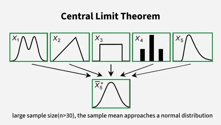
Central Limit Theorem (CLT)	For large n, the distribution of the sample mean approximates normal, regardless of the population distribution (under mild conditions).
Standard error	The standard deviation of the sample mean: σ / √n (reduces with n).

📌 1. Exact result: linear combinations of normal variables

If X_i ~ N(μ_i, σ_i²) are independent and a_i are constants, then
the linear combination S = Σ a_i X_i is normally distributed with:

Mean: E(S) = Σ a_i μ_i.
Variance: Var(S) = Σ a_i² σ_i² (independence used).
Distribution: S ~ N( Σ a_i μ_i, Σ a_i² σ_i² ).

Example:
Let X ~ N(2, 9) and Y ~ N(5, 4) independent. For T = 3X − 2Y:

E(T) = 3×2 − 2×5 = 6 − 10 = −4.

Var(T) = 3²×9 + (−2)²×4 = 9×9 + 4×4 = 81 + 16 = 97.

So T ~ N(−4, 97).

📐 IA spotlight

Use simulation to demonstrate exact normality when summing normals versus approximate normality when summing non-normal variables.
Include histograms of sums for increasing n and discuss convergence visually and numerically (mean, variance, skewness).

📌 2. Central Limit Theorem (CLT) — statement & interpretation

Let X₁, …, X_n be independent identically distributed (i.i.d.) random variables with mean μ and variance σ².
The CLT states that for large n the sample mean = (1/n)(x̄) Σ X_i is approximately normal:

(x̄)≈ N( μ, σ² / n ) for large n.

Meaning: as n increases, the distribution of the average tightens around μ and becomes bell-shaped even if the population is not normal.
How large is large? depends on population shape: for moderate skewness, n ≈ 30 is often sufficient; heavy-tail distributions require larger n.
Standard error: SE((x̄)) = σ / √n — shows how uncertainty decreases with n.

Central Limit Theorem in Statistics - GeeksforGeeks

🌍 Real-world connection

The CLT underpins why poll averages, manufacturing quality-control averages, and many sampling-based estimates can be treated using normal-approximation methods even when individual measurements are non-normal.

📌 3. Conditions, cautions and practical guidance

Independence: observations must be (approximately) independent — dependence can invalidate the CLT.
Identical distribution: not strictly necessary in more general CLT versions, but easier and common in exams.
Finite variance: the population must have finite variance for the classical CLT to apply.
Small n warning: with small n, use caution: sampling distributions may be far from normal; report this limitation in exam answers.
Skew/heavy tails: heavy-tailed distributions (e.g., Cauchy) may not converge well — discuss in words if relevant.

🧠 Paper tip — using CLT in exams

State assumptions: independence and finite variance. If n is small, explicitly say “approximation may be poor”.
Show the form: \u0305X ≈ N( μ, σ²/n ) and substitute numbers clearly. Use σ or sample s — mention which is used.
When asked for probability about sums, convert to mean form (or vice versa): sum S = n\u0305X has mean nμ and variance nσ².

Example:
Population with μ = 50, σ = 10. For n = 36, the sample mean (x̄)≈ N(50, 100/36 = 2.777…).
Standard error = 10 / √36 = 10 / 6 ≈ 1.6667.
Probability that (x̄)> 52 ≈ P( Z > (52 − 50) / 1.6667 ) = P(Z > 1.2) (use table / GDC).

🔍 TOK perspective

The CLT is a mathematical theorem but its practical truth is demonstrated by empirical convergence. What does this say about the relationship between formal proof and empirical verification in mathematics and the sciences?

🌐 EE focus

An EE could investigate empirically how large n must be for the CLT to hold for different population distributions (uniform, exponential, heavy-tailed), using simulation and metrics (KS test, skewness).

📌 4. Summary & short checklist

If the population is normal, sums/averages are exactly normal (any n).
By CLT, for large n the sample mean is approximately normal even for non-normal populations.
Use SE = σ/√n for probabilities about means, and Var(sum) = nσ² when working with sums.
Always state assumptions and comment on the quality of approximation if n is borderline.

📝 Paper strategy

Write the distribution used (exact normal or CLT approx), show formula for mean & variance, standardise using Z, and use a table or GDC for numeric probabilities.
Mention whether you used σ (population) or s (sample) and justify the choice if needed.

📌 Practice Questions: Linear Combinations & the Central Limit Theorem

Multiple Choice Questions

MCQ 1
Let X ~ N(10, 4) and Y ~ N(6, 9) be independent. Which of the following correctly describes the distribution of
T = 2X − Y?

A. T ~ N(14, 13)
B. T ~ N(14, 25)
C. T ~ N(8, 25)
D. T ~ N(8, 13)

Answer & Explanation

Correct answer: D

The mean of T is:

E(T) = 2(10) − 6 = 20 − 6 = 14 ❌ (so options C and D are eliminated?)

Wait carefully: variance first.

Var(T) = 2²(4) + (−1)²(9) = 16 + 9 = 25.

So T ~ N(14, 25). The correct option is B.

This question tests correct handling of coefficients and squaring them when computing variance.

MCQ 2
Which statement best explains why the Central Limit Theorem is important in statistics?

A. It shows that all populations are normally distributed.
B. It guarantees exact normality for any sample size.
C. It allows normal approximation for sample means from many non-normal populations.
D. It applies only when the population variance is known.

Answer & Explanation

Correct answer: C

The CLT does not claim that populations themselves are normal, nor that normality is exact for small n.
It states that the sampling distribution of the mean becomes approximately normal for large n,
regardless of population shape, provided variance is finite.

MCQ 3
For a population with mean μ and variance σ², the standard deviation of the sample mean x̄ based on n observations is:

A. σ² / n
B. σ / n
C. √(σ² / n)
D. σ / √n

Answer & Explanation

Correct answer: D

The variance of x̄ is σ² / n, so the standard deviation (standard error) is:

SE(x̄) = √(σ² / n) = σ / √n.

This reduction explains why larger samples give more precise estimates of the mean.

Short Answer Questions

Short Question 1
Explain why the variance of a linear combination of independent random variables depends on the squares of the coefficients.

Model Answer

When a random variable is multiplied by a constant a, its variance is multiplied by a².
For independent variables, variances add.
Therefore, each coefficient contributes its square to the total variance.

This reflects the fact that scaling affects spread non-linearly.

Short Question 2
State two conditions required for the Central Limit Theorem to apply reliably.

Model Answer

First, the observations must be independent.
Second, the population must have finite variance.

In practice, sufficiently large sample size is also required, especially for skewed distributions.

Long Answer Questions (IB Style)

Long Question 1

A random variable X represents the lifetime of a component with mean 120 hours and standard deviation 30 hours.
A sample of 36 components is selected.

(a) State the approximate distribution of the sample mean x̄, giving its mean and variance.
(b) Calculate the probability that the sample mean lifetime exceeds 130 hours.
(c) Comment on the validity of your method.

Full Solution

(a)

By the Central Limit Theorem, since n = 36 is reasonably large, the sampling distribution of x̄ is approximately normal.

Mean: μ = 120
Variance: σ² / n = 900 / 36 = 25

So x̄ ~ N(120, 25).

(b)

Standard deviation of x̄ = √25 = 5.

P(x̄ > 130) = P(Z > (130 − 120) / 5) = P(Z > 2).

From tables or GDC: P(Z > 2) ≈ 0.0228.

(c)

The approximation is valid provided observations are independent and the population variance is finite.
If the population distribution is highly skewed, the approximation may be weaker, but n = 36 generally gives reasonable accuracy.

Long Question 2

Independent random variables X and Y are normally distributed with:
X ~ N(50, 16), Y ~ N(30, 9).

(a) Find the distribution of S = X + Y.
(b) Find P(S > 90).
(c) Explain why no approximation is required in this question.

Full Solution

(a)

Since X and Y are independent and normal, their sum is exactly normal.

Mean: 50 + 30 = 80
Variance: 16 + 9 = 25

So S ~ N(80, 25).

(b)

Standard deviation = 5.

P(S > 90) = P(Z > (90 − 80)/5) = P(Z > 2) ≈ 0.0228.

(c)

No approximation is needed because the sum of independent normal random variables is exactly normal for any sample size.
This result does not rely on the Central Limit Theorem.